Demo: To Learn an Average, Take an Average

Roll two dice and keep the larger value: rolling with advantage. Its long-run average is \(\mu = \mathbb{E}[\max(X_1, X_2)]\).

This game is small enough to enumerate, so all \(36\) outcomes give us \(\mu\) and \(\sigma^2\) exactly.

import numpy as np
import matplotlib.pyplot as plt
import scienceplots

plt.style.use(["science", "no-latex"])
TEAL, CARDINAL = "#009090", "#9c1b33"
rng = np.random.default_rng(0)

outcomes = [(i, j) for i in range(1, 7) for j in range(1, 7)]
mu = np.mean([max(i, j) for i, j in outcomes])
sigma2 = np.mean([(max(i, j) - mu) ** 2 for i, j in outcomes])
print(f"exact mean      mu      = {mu:.4f}  (= 161/36)")
print(f"exact variance  sigma^2 = {sigma2:.4f}  (= 2555/1296)")
print(f"one-game spread sigma   = {np.sqrt(sigma2):.4f}")

exact mean      mu      = 4.4722  (= 161/36)
exact variance  sigma^2 = 1.9715  (= 2555/1296)
one-game spread sigma   = 1.4041

Now pretend we can’t enumerate: twenty dice, rerolls, a rulebook of modifiers, or a model’s error on every photo on the internet. We can still play. The Monte Carlo estimator plays \(n\) games and averages them:

\[\hat{\mu}_n = \frac{1}{n}\sum_{i=1}^n f(X^{(i)}), \qquad f(X) = \max(X_1, X_2),\]

where \(X^{(i)}\) is the \(i\)-th game, a fresh pair of dice. In class we proved this is unbiased, and lecture also predicts its error: \(\sigma/\sqrt{n} \approx 1.40/\sqrt{n}\).

Before running: how many games do we need for one decimal place of accuracy? For two?

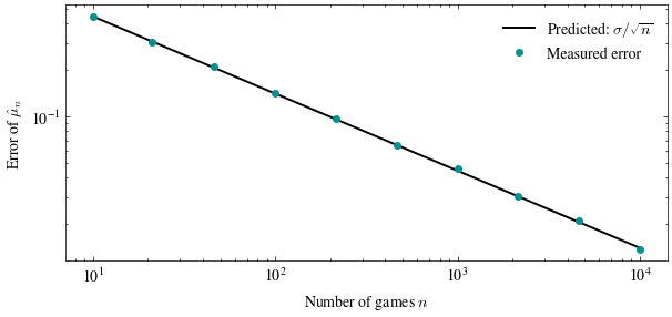
ns = np.unique(np.logspace(1, 4, 10).astype(int))
reps = 1000  # replay each experiment many times to measure the typical error

errors = []
for n in ns:
    dice = rng.integers(1, 7, size=(reps, n, 2), dtype=np.int8)
    estimates = dice.max(axis=2).mean(axis=1)
    errors.append(estimates.std())

fig, ax = plt.subplots(figsize=(7, 3))
ax.loglog(ns, np.sqrt(sigma2 / ns), color="black", linewidth=1.4,
          label=r"Predicted: $\sigma/\sqrt{n}$")
ax.loglog(ns, errors, "o", color=TEAL, markersize=4, label="Measured error")
ax.set_xlabel(r"Number of games $n$")
ax.set_ylabel(r"Error of $\hat{\mu}_n$")
ax.legend(frameon=False)
plt.show()

A straight line of slope \(-\frac{1}{2}\) on log-log axes: the \(1/\sqrt{n}\) rate, exactly as predicted. Each extra digit of accuracy costs \(100\times\) more games. Expensive.

Same samples, better answer

The sum of the two dice is a surrogate with a known mean: \(\mathbb{E}[X_1 + X_2] = 7\) by linearity, with no enumeration at all. When the sum runs high the max probably runs high too, so subtract off the measured luck:

\[\hat{\mu}_c = \frac{1}{n}\sum_{i=1}^n \left[ f(X^{(i)}) - c\,\big(g(X^{(i)}) - 7\big) \right], \qquad g(X) = X_1 + X_2.\]

In class we proved this is unbiased for every \(c\). Guess \(c = \tfrac{1}{2}\), since the max is roughly half the sum.

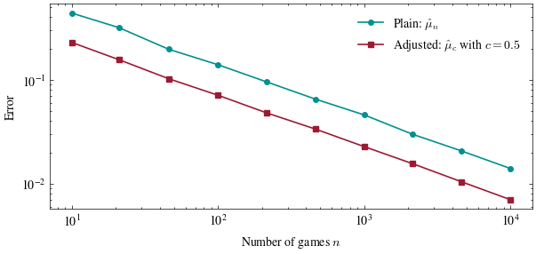
c = 0.5

errors_plain, errors_adj = [], []
for n in ns:
    dice = rng.integers(1, 7, size=(reps, n, 2), dtype=np.int8)
    maxes, sums = dice.max(axis=2), dice.sum(axis=2)
    errors_plain.append(maxes.mean(axis=1).std())
    errors_adj.append((maxes - c * (sums - 7)).mean(axis=1).std())

fig, ax = plt.subplots(figsize=(7, 3))
ax.loglog(ns, errors_plain, "o-", color=TEAL, markersize=4, linewidth=1.2,
          label=r"Plain: $\hat{\mu}_n$")
ax.loglog(ns, errors_adj, "s-", color=CARDINAL, markersize=4, linewidth=1.2,
          label=rf"Adjusted: $\hat{{\mu}}_c$ with $c = {c}$")
ax.set_xlabel(r"Number of games $n$")
ax.set_ylabel("Error")
ax.legend(frameon=False)
plt.show()

Parallel lines, but the adjusted one runs about \(2\times\) lower: the same samples, the accuracy of \(4n\) games. No new rolls were needed, only arithmetic on side information we already had.

What if we change \(c\)?

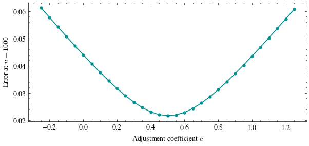
Is \(c = \tfrac{1}{2}\) the best we can do? Try other values, including negative ones and large ones.

cs = np.linspace(-0.25, 1.25, 31)
n = 1000

dice = rng.integers(1, 7, size=(reps, n, 2), dtype=np.int8)
maxes, sums = dice.max(axis=2), dice.sum(axis=2)
errors_c = [(maxes - c * (sums - 7)).mean(axis=1).std() for c in cs]

fig, ax = plt.subplots(figsize=(7, 3))
ax.plot(cs, errors_c, "o-", color=TEAL, markersize=3.5, linewidth=1.2)
ax.set_xlabel(r"Adjustment coefficient $c$")
ax.set_ylabel(rf"Error at $n = {n}$")
plt.show()

Punchline: any quantity that is correlated with the target and has a known mean is free variance reduction.

The error traces a curve with a bottom. Problem 2 finds that bottom in closed form and shows that the correlation \(\rho\) between \(f\) and \(g\) sets exactly how much the adjustment can save. Correlation inflated the variance of a sum last week; here it shrinks the estimator’s variance instead.