Monte Carlo Estimator
Last lecture, we built a language for randomness: events, random variables, expectation, variance, and covariance. Today, we spend that vocabulary on the course’s first and simplest algorithm: to learn an average, take an average.
Why do we care about averages? Because most of the quantities machine learning cares about are expectations. The training loss we will minimize all semester is an average over a dataset far too large to touch every example at every step. The score of a game-playing agent is the expected outcome over the randomness of the game. Neither can be computed exactly, but both can be sampled. So the question of the day is:
By the end of the lecture we will know the answer exactly, and it will depend on only two things: how many samples we draw, and how much a single sample varies. More samples are expensive, so the second is where the rest of the course spends its cleverness.
Rolling with Advantage
Here is a game: roll two fair six-sided dice and keep the larger of the two values. Tabletop gamers call this rolling with advantage. It certainly feels better than rolling one die, but how much better, on average? Let \(X_1\) and \(X_2\) be the two rolls, the same two dice we met last lecture, so that a single game is the pair \(X = (X_1, X_2)\) and the value we keep is \(f(X) = \max(X_1, X_2)\). The number we are after is the long-run average value kept: \[ \mu = \mathbb{E}[\max(X_1, X_2)]. \]
For this tiny game, we can compute \(\mu\) exactly by enumerating the \(6 \times 6 = 36\) equally likely outcomes. The maximum is at most \(k\) exactly when both dice are at most \(k\), and the two rolls are independent, so those two conditions multiply: \[ \Pr(\max(X_1, X_2) \leq k) = \frac{k}{6} \cdot \frac{k}{6} = \frac{k^2}{36}. \] Subtracting consecutive values of that expression leaves the probability of landing on \(k\) exactly: \[ \Pr(\max(X_1, X_2) = k) = \frac{k^2 - (k-1)^2}{36} = \frac{2k - 1}{36}. \] Weighting each value by its probability gives the expectation we came for: \[ \mu = \sum_{k=1}^6 k \cdot \frac{2k-1}{36} = \frac{1 + 6 + 15 + 28 + 45 + 66}{36} = \frac{161}{36} \approx 4.47. \]
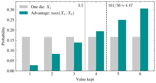
In the plot, advantage drags the distribution to the right: the flat gray distribution of a single die becomes a ramp that favors large values, and the mean climbs from \(3.5\) to about \(4.47\).
Enumeration worked because the game was tiny. Replace two dice with twenty, add rerolls and a rulebook of modifiers, and the number of outcomes explodes. Replace the game with “the error of a model on a random photo from the internet” and enumeration is not even meaningful. But notice what survives: even when we cannot enumerate the game, we can still play it.
The Sample Mean Estimator
Let’s set up the general problem. There is a random variable \(X\) (possibly a vector, like an image or a whole game), and a function \(f\) that scores it with a real number. The quantity we want is the average score: \[ \mu = \mathbb{E}[f(X)]. \] We cannot evaluate that expectation, but we can draw \(n\) independent samples \(X^{(1)}, \ldots, X^{(n)}\), each distributed like \(X\), and report their sample mean. This rule is the Monte Carlo estimator: \[ \hat{\mu}_n = \frac{1}{n} \sum_{i=1}^n f(X^{(i)}). \] An estimator is any rule that turns samples into a guess for an unknown quantity; this one is named after the casino in Monaco. In the advantage roll, \(X^{(i)}\) is the \(i\)-th game, a fresh pair of dice, and \(f(X^{(i)})\) is the larger of that pair. The parenthesized superscript indexes samples, and it is the notation we will use for data points all semester.
Two questions decide whether an estimator is any good. Does it point at the right target? And how quickly does it get there as we collect samples?
Correct on Average
The first question’s answer is the reason we spent last lecture on linearity of expectation. The mechanical reason is that an average of \(n\) quantities, each of which is right on average, is itself right on average; nothing about how the samples interact can move the center.
Claim: The Monte Carlo estimator is correct on average: \(\mathbb{E}[\hat{\mu}_n] = \mu\).
Proof of Claim
Each sample is distributed like \(X\), so \(\mathbb{E}[f(X^{(i)})] = \mu\) for every \(i\). By linearity of expectation, the constant \(\frac1n\) slides out and the expectation of the sum is the sum of the expectations: \[ \mathbb{E}[\hat{\mu}_n] = \frac{1}{n} \sum_{i=1}^n \mathbb{E}[f(X^{(i)})] = \frac{1}{n} \cdot n \mu = \mu. \] Notice that we never used independence. Linearity of expectation holds no matter how the samples relate, so even badly correlated samples still give an unbiased estimate; they just give a worse one.An estimator whose expectation equals its target is called unbiased: its errors have no systematic direction. Unbiasedness alone is a low bar, though. The lazy rule “play one game and report it” is also unbiased, but nobody would trust it. What separates the sample mean from the lazy rule is the second question: variance.
The \(1/\sqrt{n}\) Rate
Variance is where independence finally matters. Let \(\sigma^2\) be the variance of a single sample’s score: \[ \sigma^2 = \textnormal{Var}(f(X)). \] Because the samples are independent, every covariance term in last lecture’s variance-of-a-sum formula is zero, so the \(n\) variances simply add. The \(\frac1n\) out front then comes back out squared, dividing by \(n^2\) rather than by \(n\), and the mismatch between those two powers is the entire result: \[ \textnormal{Var}(\hat{\mu}_n) = \frac{\sigma^2}{n}. \] Problem 1 has you carry out this calculation in full, and then discover what happens to it when independence fails.
The error we should typically expect is the standard deviation, which is the square root of that variance: \[ \sqrt{\textnormal{Var}(\hat{\mu}_n)} = \frac{\sigma}{\sqrt{n}}. \] It shrinks to zero as \(n\) grows, which is the law of large numbers with a rate attached, and we call it the \(1/\sqrt{n}\) rate. The square root in the denominator is the bad news: halving the error takes four times the samples, and each extra decimal digit of accuracy takes a factor of one hundred more games. The numerator is the good news, because \(\sigma\) is the only feature of the problem that the formula mentions. How complicated \(f\) is, how many dice are on the table, how many dimensions \(X\) lives in: none of it enters except through the spread of a single game.
For the advantage roll, enumeration gives \(\sigma^2 = \frac{2555}{1296} \approx 1.97\), so \(\sigma \approx 1.40\), and the formula predicts an error near \(1.40/\sqrt{100} = 0.14\) after \(100\) games and near \(0.014\) after \(10{,}000\). The class demo plays the game at each \(n\) and checks that the measured error lands on this prediction.
A hundred times the games for one more digit is a bad deal; would we do better by not sampling at all?
Any Dimension You Like
A \(1/\sqrt{n}\) rate may look slow until you see what it replaces. The deterministic alternative to sampling is a grid: to average a function over a square, evaluate it at every point of a \(20 \times 20\) lattice and average the \(400\) values. In two dimensions, that works fine. But the cost of a grid is \(m^d\) evaluations for \(m\) points per axis in \(d\) dimensions: at \(d = 10\) our modest grid already needs \(20^{10} \approx 10^{13}\) points, and the quantities we will meet later in the course live in millions of dimensions. This exponential blow-up is called the curse of dimensionality, and it kills the grid.
The Monte Carlo estimator does not: its error is \(\sigma/\sqrt{n}\), and that formula never mentions \(d\). A classic example is estimating \(\pi\) by throwing darts: let \(X\) be a uniformly random point in the unit square and \(f(X)\) the indicator that \(X\) lands inside the quarter circle, so that \(\mu = \mathbb{E}[f(X)] = \pi/4\). The exact same code estimates the volume of a ball in \(100\) dimensions, where no grid could ever go. (\(\sigma\) itself can grow with the problem; the rate \(1/\sqrt{n}\) does not.)
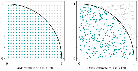
In the plot, both panels spend the same budget of \(400\) points to estimate the quarter circle’s area: the grid on the left is beautifully organized, the darts on the right are a mess, and both land within a couple percent of \(\pi\).
In high dimensions, then, sampling is the only method still standing, so if we want a better answer, its error formula is what we have to attack.
Control Variate
Now for the nagging issue. The error \(\sigma/\sqrt{n}\) has two knobs, and the \(n\) knob is expensive. The other knob is \(\sigma\), the spread of a single game. Can we shrink that instead?
Here is the idea. Suppose that alongside our target \(f(X)\) there is a surrogate quantity \(g(X)\) with two properties: it is correlated with \(f(X)\), and we know its expectation \(\mathbb{E}[g(X)]\) exactly. For the advantage roll, the surrogate is already sitting on the table: take \(g(X) = X_1 + X_2\), the sum of the same two dice. Last lecture, linearity of expectation gave us \(\mathbb{E}[X_1 + X_2] = 7\) with no enumeration at all, and the sum is clearly correlated with the max, since a high sum usually means a high larger die.
The control variate adjustment subtracts the surrogate’s measured luck: \[ \hat{\mu}_c = \frac{1}{n} \sum_{i=1}^n \Big[ f(X^{(i)}) - c \big( g(X^{(i)}) - \mathbb{E}[g(X)] \big) \Big], \] where \(c\) is a constant we get to choose. (The subscript on \(\hat{\mu}_c\) names that coefficient rather than a sample count; we still draw \(n\) samples.) The correction term \(g(X^{(i)}) - \mathbb{E}[g(X)]\) measures which way the luck ran on game \(i\). If the dice summed above \(7\), the rolls ran lucky, the recorded max is probably an overestimate, and the adjustment pulls it back down by \(c\) times the measured luck.
Adjusting our estimates by something random sounds dangerous. Could it drag the estimator off target? It cannot, and this was our second in-class exercise.
Claim: The adjusted estimator is unbiased for every choice of \(c\): \(\mathbb{E}[\hat{\mu}_c] = \mu\).
Proof of Claim
By linearity of expectation, we can take the expectation of each piece separately: \[ \mathbb{E}[\hat{\mu}_c] = \frac{1}{n} \sum_{i=1}^n \Big( \mathbb{E}[f(X^{(i)})] - c \big( \mathbb{E}[g(X^{(i)})] - \mathbb{E}[g(X)] \big) \Big) = \frac{1}{n} \sum_{i=1}^n \big( \mu - c \cdot 0 \big) = \mu, \] where each correction term vanishes because \(X^{(i)}\) is distributed like \(X\), so \(\mathbb{E}[g(X^{(i)})] = \mathbb{E}[g(X)]\). This is why the surrogate’s mean must be known: we subtract the true mean, not a guess, and the correction is centered exactly at zero.So the choice of \(c\) costs us nothing in bias; it only changes the variance. Setting \(c = 0\) recovers the plain estimator, so the adjusted family can only do as well or better, provided we choose \(c\) well. Let’s try a guess. The larger of two dice is roughly half their sum, so take \(c = \frac12\). Enumeration gives the variance of a single adjusted sample as \(\frac{665}{1296} \approx 0.51\), down from \(\sigma^2 \approx 1.97\). That is nearly a factor of four less variance, and since the error is the square root of the variance, it is half the error at every single \(n\): with \(n\) games the adjusted estimator reaches what the plain one needs about \(4n\) to match.
Is \(\frac12\) the best possible choice? That is Problem 2. You will show that the variance of \(\hat{\mu}_c\) is a parabola in \(c\), find the bottom of the parabola in closed form, and discover that the size of the reduction is set exactly by the correlation \(\rho\) between \(f(X)\) and \(g(X)\), the covariance divided by the two standard deviations from last lecture. It is the same \(\rho\) that put a floor under the poll in Problem 1: correlation worked against us there and works for us here.
Looking Forward
Today introduced a theme we return to for the rest of the semester: variance reduction. When we train neural networks, stochastic gradient descent will turn out to be a Monte Carlo estimator of the true gradient, with the batch playing the role of the samples. And in the final week, an agent learning from rewards will estimate its expected return by Monte Carlo and reduce the variance by subtracting a baseline, which is today’s adjustment down to the exact coefficient you derive on Problem 2.
Next lecture, we set randomness aside and pick up the second toolbox of this unit: linear algebra, the language in which data and models are written.
If you carry one sentence out of today, carry this one: when part of what you are measuring is something whose average you already know, subtract that part off and spend your samples on the rest.