Linear Algebra
When I first heard about machine learning, I imagined a computer rewarded with electric carrots and sticks; in fact machine learning runs on mathematics, and the mathematics is linear algebra.
We have spent two lectures on randomness: a language for uncertainty, and an estimator that turns samples into answers. Today we collect the unit’s second toolbox, the language data and models are written in. A dataset will be a matrix, a model’s parameters a vector, and a prediction an inner product. Everything we build on them comes back to one question:
The answer we build toward is that a matrix is a function, and that reading a matrix means reading its columns. We open with derivatives, which look like a different subject but are not: the gradient is defined through an inner product, and to first order a derivative is a linear map.
Derivatives
Consider a function \(f: \mathbb{R} \to \mathbb{R}\), mapping a single real number to a single real number. Mathematicians tell us to be careful about whether we can differentiate; we’re computer scientists, so we’ll risk it for the biscuit.
The derivative of \(f\) at \(x\) is the limiting slope of a shrinking secant line: \[ f'(x) = \frac{\partial}{\partial x}[f(x)] = \lim_{h \to 0} \frac{f(x + h) - f(x)}{h}. \] Read it as a rate of response: nudge the input by a tiny \(h\), and the output moves by about \(f'(x) \cdot h\); every optimization algorithm in this course hunts for the flat spots where the derivative vanishes. Here are the derivatives we will use most often.
| Function: \(f(x)\) | Derivative: \(f'(x)\) |
| \[ax + b\] | \[a\] |
| \[x^a\] | \[a x^{a-1}\] |
| \[\ln(x)\] | \[\frac{1}{x}\] |
| \[e^x\] | \[e^x\] |
Two rules let us differentiate functions built from simpler pieces. For another function \(g: \mathbb{R} \to \mathbb{R}\), the chain rule handles composition: \[ \frac{\partial}{\partial x}[g(f(x))] = g'(f(x)) \, f'(x). \] And the product rule handles multiplication: \[ \frac{\partial}{\partial x}[g(x) f(x)] = g(x) f'(x) + f(x) g'(x). \] The chain rule says a composition’s sensitivity is the product of its links’ sensitivities: a nudge to \(x\) is amplified by \(f'(x)\) on the way in and by \(g'\) on the way out. Modern machine learning composes thousands of functions, and differentiating one link at a time is precisely what backpropagation will do in the Neural Networks unit, one matrix per link.
Both rules describe a function of a single input; machine learning models have millions, so we need a derivative that handles them all at once.
Gradients
Consider \(f: \mathbb{R}^d \to \mathbb{R}\), whose input \(\mathbf{x} \in \mathbb{R}^d\) collects the \(d\) real numbers \(x_1, \ldots, x_d\). The partial derivative \(\frac{\partial}{\partial x_i}[f(\mathbf{x})]\) measures how \(f\) changes when we nudge \(x_i\), holding the other inputs fixed. The gradient stacks all \(d\) partial derivatives into a vector: \[ \nabla_\mathbf{x} f = \begin{bmatrix} \frac{\partial}{\partial x_1}[f(\mathbf{x})] \\ \vdots \\ \frac{\partial}{\partial x_d}[f(\mathbf{x})] \end{bmatrix}. \]
The description we will lean on mentions no coordinates: stand at \(\mathbf{x}\), step a tiny distance \(\epsilon\) in the direction \(\mathbf{v} \in \mathbb{R}^d\), and \(f\) responds according to the directional definition of the gradient: \[ f(\mathbf{x} + \epsilon \mathbf{v}) = f(\mathbf{x}) + \epsilon \, \langle \nabla_\mathbf{x} f, \mathbf{v} \rangle + o(\epsilon), \] where \(\langle \cdot, \cdot \rangle\) is the inner product defined in the next section and \(o(\epsilon)\) collects terms that shrink faster than \(\epsilon\), like \(\epsilon^2\). The formula says the whole first-order behavior of \(f\) at \(\mathbf{x}\) is carried by the single vector \(\nabla_\mathbf{x} f\): the response is largest along the gradient, zero orthogonal to it, and most negative against it, which is why gradient descent steps in the direction \(-\nabla_\mathbf{x} f\). Problem 3 uses exactly this definition to derive the three gradients we will use all semester, so it is the problem you will cite most often.
We have leaned on the inner product twice without defining it, so let’s collect the vector vocabulary.
Vectors, Inner Products, and Norms
Consider two vectors \(\mathbf{u}, \mathbf{v} \in \mathbb{R}^d\). Their inner product is the sum of their entrywise products: \[ \langle \mathbf{u}, \mathbf{v} \rangle = \mathbf{u}^\top \mathbf{v} = \sum_{i=1}^d u_i v_i, \] where \(\mathbf{u}^\top \in \mathbb{R}^{1 \times d}\) is the transpose of \(\mathbf{u}\), the same numbers laid on their side. The inner product measures alignment: large and positive when the vectors point the same way, zero when they are orthogonal (perpendicular), and negative when they oppose; forming it costs \(O(d)\) operations.
Taking the inner product of a vector with itself gives the squared length, and its square root is the norm: \[ \|\mathbf{v}\|_2 = \sqrt{\langle \mathbf{v}, \mathbf{v} \rangle} = \sqrt{\textstyle\sum_{i=1}^d v_i^2}, \] generalizing the Pythagorean theorem to \(d\) dimensions.
One family of vectors deserves a name: the standard basis vectors \(\mathbf{e}_1, \ldots, \mathbf{e}_d\), where \(\mathbf{e}_k \in \mathbb{R}^d\) has a \(1\) in position \(k\) and \(0\) everywhere else. Every vector is a recipe of them, with its entries as the amounts: \[ \mathbf{x} = \sum_{k=1}^d x_k \mathbf{e}_k. \] Keep them in mind; they are about to tell us how to read a matrix.
A Matrix Is a Map
A matrix \(\mathbf{A} \in \mathbb{R}^{n \times d}\) is usually introduced as a grid of numbers, but the productive view is that \(\mathbf{A}\) is a function: it eats a vector \(\mathbf{x} \in \mathbb{R}^d\) and outputs \(\mathbf{A}\mathbf{x} \in \mathbb{R}^n\), whose \(i\)th entry is the inner product of the \(i\)th row with \(\mathbf{x}\). The equivalent description to memorize: substituting the basis expansion \(\mathbf{x} = \sum_k x_k \mathbf{e}_k\) and pushing \(\mathbf{A}\) through the sum shows the output is a recipe mixing the columns of \(\mathbf{A}\), with the entries of \(\mathbf{x}\) as the amounts: \[ \mathbf{A}\mathbf{x} = \sum_{k=1}^d x_k [\mathbf{A}]_{,k}, \] where \([\mathbf{A}]_{,k} \in \mathbb{R}^n\) denotes the \(k\)th column. Pushing \(\mathbf{A}\) through a sum is allowed because \(\mathbf{x} \mapsto \mathbf{A}\mathbf{x}\) is a linear map, respecting scaling and addition for all vectors \(\mathbf{u}, \mathbf{v} \in \mathbb{R}^d\) and scalars \(\alpha, \beta\): \[ \mathbf{A}(\alpha \mathbf{u} + \beta \mathbf{v}) = \alpha \mathbf{A}\mathbf{u} + \beta \mathbf{A}\mathbf{v}. \] Geometrically, the map sends lines to lines, holds the origin fixed, and warps space without tearing or bending it.
Where do the basis vectors land? Feeding \(\mathbf{e}_k\) into the recipe kills every term but one: \[ \mathbf{A}\mathbf{e}_k = \sum_{j=1}^d [\mathbf{e}_k]_j \, [\mathbf{A}]_{,j} = [\mathbf{A}]_{,k}. \] So the columns of a matrix are exactly where it sends the basis vectors. To read a matrix, read its columns.
Today’s examples are four matrices in \(\mathbb{R}^{2 \times 2}\), all doing the same job of moving the plane, so they share the name \(\mathbf{A}\) and differ only by a tag. The first two are a rotation by \(\theta\) and a coordinate-wise stretch: \[ \mathbf{A}^{\mathrm{rot}} = \begin{bmatrix} \cos\theta & -\sin\theta \\ \sin\theta & \cos\theta \end{bmatrix} \qquad \text{and} \qquad \mathbf{A}^{\mathrm{scale}} = \begin{bmatrix} 2 & 0 \\ 0 & \frac12 \end{bmatrix}. \] Read the columns and the pictures follow: \(\mathbf{A}^{\mathrm{rot}}\)’s columns are the basis vectors rotated by \(\theta\), so the plane turns by \(\theta\); \(\mathbf{A}^{\mathrm{scale}}\) pulls the plane out by \(2\) horizontally and squashes it by \(\frac12\) vertically.
The third example is the in-class exercise, a shear: \[ \mathbf{A}^{\mathrm{shear}} = \begin{bmatrix} 1 & 1 \\ 0 & 1 \end{bmatrix}. \] Its columns say that \(\mathbf{e}_1\) does not move while \(\mathbf{e}_2\) tips a full unit right: squares lean into parallelograms.
Solution to the class exercise
Push the basis vectors through it and read the answer off the columns: \[ \mathbf{A}^{\mathrm{shear}} \mathbf{e}_1 = \begin{bmatrix} 1 \\ 0 \end{bmatrix} = \mathbf{e}_1, \qquad \mathbf{A}^{\mathrm{shear}} \mathbf{e}_2 = \begin{bmatrix} 1 \\ 1 \end{bmatrix}. \] So \(\mathbf{e}_2\) keeps its height while tipping right, and every horizontal line slides along itself, because a point at height \(x_2\) is pushed right by exactly \(x_2\).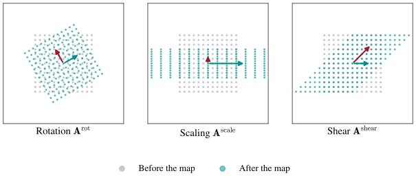
In the plot, each panel applies one of the three matrices to the same grid, the two arrows again the images of \(\mathbf{e}_1\) and \(\mathbf{e}_2\); the shear panel on the right matches the exercise above, \(\mathbf{e}_2\) tipping right while \(\mathbf{e}_1\) holds still.
Every map so far has been reversible: rotate back, squash back, unlean the parallelograms. The fourth one will not be, and the reason is the subject of the next section.
Column Space and Rank
Since \(\mathbf{A}\mathbf{x}\) is always a mix of columns, the set of all possible outputs of the map is the set of all such mixes: the column space of \(\mathbf{A}\). Its dimension is the rank of \(\mathbf{A}\), equivalently the number of linearly independent columns.
Rank measures how much of the output space the map can reach; the fastest way to shrink it is to make one column a multiple of another. Here is the fourth example matrix, whose second column is exactly twice its first: \[ \mathbf{A}^{\mathrm{flat}} = \begin{bmatrix} 1 & 2 \\ \frac12 & 1 \end{bmatrix}. \] Expanding an output in the column recipe and factoring out the shared column shows where every output must live: \[ \mathbf{A}^{\mathrm{flat}} \mathbf{x} = x_1 \begin{bmatrix} 1 \\ \frac12 \end{bmatrix} + x_2 \begin{bmatrix} 2 \\ 1 \end{bmatrix} = x_1 \begin{bmatrix} 1 \\ \frac12 \end{bmatrix} + 2 x_2 \begin{bmatrix} 1 \\ \frac12 \end{bmatrix} = (x_1 + 2 x_2) \begin{bmatrix} 1 \\ \frac12 \end{bmatrix}. \] Whatever \(\mathbf{x}\) we feed in, the output is some multiple of the single vector \((1, \frac12)\), so two dimensions of input are flattened onto one line of output and \(\mathbf{A}^{\mathrm{flat}}\) has rank \(1\).
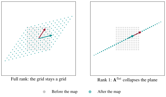
In the plot, a full-rank matrix on the left warps the gray grid into a teal parallelogram that is still two-dimensional, while \(\mathbf{A}^{\mathrm{flat}}\) on the right crushes the same grid onto the line through \((1, \frac12)\); the class demo runs this same collapse on a photograph.
Rank matters to us because collapse destroys information: every input on the line \(x_1 + 2x_2 = 0\) is sent to the origin, and no later procedure can tell those inputs apart. When we fit linear models, the question “which predictions can our model even produce?” will be, word for word, “what is the column space of the data matrix?”
So far we have applied one map at a time. What happens when we apply two in a row?
Matrix Multiplication, Two Ways
Consider matrices \(\mathbf{A} \in \mathbb{R}^{n \times m}\) and \(\mathbf{B} \in \mathbb{R}^{m \times d}\). The product \(\mathbf{A}\mathbf{B}\) is the matrix of the composed map, first \(\mathbf{B}\) then \(\mathbf{A}\), so it is only defined when the inner dimensions agree: \(\mathbf{B}\) must land in the space \(\mathbf{A}\) eats from. The familiar formula computes each entry as an inner product of a row of \(\mathbf{A}\) with a column of \(\mathbf{B}\): \[ [\mathbf{A}\mathbf{B}]_{i,j} = \sum_{k=1}^m [\mathbf{A}]_{i,k} [\mathbf{B}]_{k,j}. \]
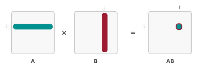
In the diagram, one entry is highlighted along with the two slices that produce it: row \(i\) of \(\mathbf{A}\) and column \(j\) of \(\mathbf{B}\); each of the \(nd\) entries costs \(m\) multiplications, so the whole product costs \(O(nmd)\).
There is a second way to organize the very same sum. For a column vector \(\mathbf{u} \in \mathbb{R}^n\) and a row vector \(\mathbf{v}^\top \in \mathbb{R}^{1 \times d}\), their outer product is the \(n \times d\) matrix whose \((i,j)\) entry is \(u_i v_j\): \[ \mathbf{u}\mathbf{v}^\top \in \mathbb{R}^{n \times d}, \qquad [\mathbf{u}\mathbf{v}^\top]_{i,j} = u_i v_j. \] Every column of \(\mathbf{u}\mathbf{v}^\top\) is a multiple of \(\mathbf{u}\), so the outer product of two nonzero vectors has rank \(1\): a whole matrix built from one column and one row. Grouping the entry formula by \(k\) instead of by \((i,j)\) writes matrix multiplication as a sum of such pieces, one per inner index: \[ \mathbf{A}\mathbf{B} = \sum_{k=1}^m [\mathbf{A}]_{,k} [\mathbf{B}]_{k,}, \] where \([\mathbf{B}]_{k,} \in \mathbb{R}^{1 \times d}\) denotes the \(k\)th row of \(\mathbf{B}\).
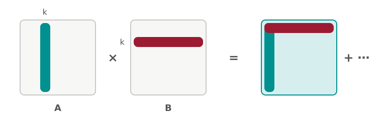
In the diagram, column \(k\) of \(\mathbf{A}\) and row \(k\) of \(\mathbf{B}\) produce one full-size rank-\(1\) matrix, and the product is the sum of \(m\) of them: the entry form builds the answer one pixel at a time, the outer-product form one layer at a time.
You may reasonably object that a second name for one sum is not progress. The payoff is that layers can be ranked and pixels cannot. Every term \([\mathbf{A}]_{,k}[\mathbf{B}]_{k,}\) is a complete matrix of the right shape, so we can ask which layers carry most of the product and discard the rest, whereas a single entry of the product means nothing on its own. That is next lecture’s main tool: the singular value decomposition writes a matrix as a sum of rank-\(1\) layers ordered from most to least important, and keeping only the first few is how we will compress images, denoise data, and finetune large models.
The in-class exercise checks that the two forms agree on a small example: \[ \begin{bmatrix} 1 & 2 \\ 3 & 4 \end{bmatrix} \begin{bmatrix} 5 & 6 \\ 7 & 8 \end{bmatrix} = \begin{bmatrix} 19 & 22 \\ 43 & 50 \end{bmatrix} \] by either route, with the \((2,1)\) entry arriving as \(3 \cdot 5 + 4 \cdot 7 = 43\) and as \(15 + 28\) from the rank-\(1\) layers.
Solution to the class exercise
The outer-product form adds one rank-\(1\) layer per inner index: \[ \begin{bmatrix} 1 & 2 \\ 3 & 4 \end{bmatrix} \begin{bmatrix} 5 & 6 \\ 7 & 8 \end{bmatrix} = \begin{bmatrix} 1 \\ 3 \end{bmatrix} \begin{bmatrix} 5 & 6 \end{bmatrix} + \begin{bmatrix} 2 \\ 4 \end{bmatrix} \begin{bmatrix} 7 & 8 \end{bmatrix} = \begin{bmatrix} 5 & 6 \\ 15 & 18 \end{bmatrix} + \begin{bmatrix} 14 & 16 \\ 28 & 32 \end{bmatrix} = \begin{bmatrix} 19 & 22 \\ 43 & 50 \end{bmatrix}. \] Naming the two factors \(\mathbf{A}\) and \(\mathbf{B}\), the entry form reaches the same place by taking a row of the first against a column of the second: \[ [\mathbf{A}\mathbf{B}]_{2,1} = 3 \cdot 5 + 4 \cdot 7 = 43, \] the same \(43\) that showed up as \(15 + 28\) in the layers.Rearranging the sum changes what we can see in it, never the arithmetic or its \(O(nmd)\) cost.
Composition builds maps up. Can we take them apart again?
Transpose, Identity, and Inverse
Three pieces of bookkeeping complete the toolbox. The transpose \(\mathbf{A}^\top\) swaps rows and columns, so \([\mathbf{A}^\top]_{i,j} = [\mathbf{A}]_{j,i}\); in particular the \(i\)th row of \(\mathbf{A}\), stood up as a column, is \(\mathbf{a}_i = ([\mathbf{A}]_{i,})^\top\). That is the notation Problem 3 uses when it expands \(\mathbf{A}^\top\mathbf{A}\) as a sum of outer products. Transposing a product reverses its order: \[ (\mathbf{A}\mathbf{B})^\top = \mathbf{B}^\top \mathbf{A}^\top. \] A square matrix equal to its own transpose is symmetric; symmetric matrices get a lecture of their own next time. The identity matrix \(\mathbf{I}_d \in \mathbb{R}^{d \times d}\), with ones on the diagonal and zeros elsewhere, is the do-nothing map: \(\mathbf{I}_d \mathbf{x} = \mathbf{x}\) for every \(\mathbf{x}\).
The inverse of a square matrix \(\mathbf{A} \in \mathbb{R}^{d \times d}\), when it exists, is the matrix \(\mathbf{A}^{-1}\) that undoes the map: \[ \mathbf{A}^{-1} \mathbf{A} = \mathbf{A} \mathbf{A}^{-1} = \mathbf{I}_d. \] It is the tool that solves equations: if \(\mathbf{A}\mathbf{x} = \mathbf{b}\), then \(\mathbf{x} = \mathbf{A}^{-1}\mathbf{b}\), the matrix version of dividing both sides of \(ax = b\) by \(a\). Rank tells us exactly which square matrices have an inverse: precisely those with full rank \(d\). Our rank-\(1\) matrix \(\mathbf{A}^{\mathrm{flat}}\) flattened the plane onto a line, so many inputs share each output. Do you see why no function, matrix or otherwise, could undo that?
One inverse is free: the rotation \(\mathbf{A}^{\mathrm{rot}}\) is undone by its transpose, and matrices with that property, called orthogonal, star in the next lecture. In general, computing an inverse costs \(O(d^3)\) time, as does solving \(\mathbf{A}\mathbf{x} = \mathbf{b}\) directly; that cost returns when we fit our first model and must decide whether we can afford the exact answer.
Looking Forward
Both toolboxes of the unit are now open: probability for randomness, linear algebra for data and transformations. Problem 3 joins today’s two halves, using the inner-product definition of the gradient to differentiate the matrix expressions every later lecture minimizes; its closing quadratic form reveals the shape of the least-squares loss, the reason gradient descent works.
Next lecture asks whether a matrix has special directions it only stretches, without rotating. Chasing them leads to eigenvectors and the singular value decomposition, which writes every matrix as a rotation, a stretch, and a rotation in today’s outer-product notation.
If you carry one sentence out of today, carry this one: to find out what a linear map does, ask where it sends the basis vectors, and read the answer off the columns.