Demo: The Power Method

Last lecture, every matrix we applied rotated and stretched the grid. Today we hunt for the directions a matrix only stretches, its eigenvectors, with a single move applied over and over: multiply, normalize, repeat.

Our running example from lecture: \[\mathbf{A} = \begin{bmatrix} 2 & 1 \\ 1 & 2 \end{bmatrix}, \qquad \mathbf{v}_1 = \tfrac{1}{\sqrt 2}(1,1) \text{ with } \lambda_1 = 3, \qquad \mathbf{v}_2 = \tfrac{1}{\sqrt 2}(1,-1) \text{ with } \lambda_2 = 1.\]

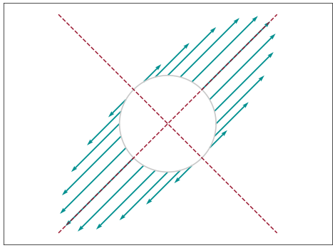
First, a picture of what \(\mathbf{A}\) does to every direction at once: at each point \(\mathbf{x}\) on the unit circle, draw the arrow from \(\mathbf{x}\) to \(\mathbf{A}\mathbf{x}\).

import numpy as np
import matplotlib.pyplot as plt
import scienceplots

plt.style.use(["science", "no-latex"])
TEAL, CARDINAL, GRAY = "#009090", "#9c1b33", "#c9c9c9"

A = np.array([[2.0, 1.0], [1.0, 2.0]])
v1 = np.array([1.0, 1.0]) / np.sqrt(2)
v2 = np.array([1.0, -1.0]) / np.sqrt(2)

t = np.linspace(0, 2 * np.pi, 24, endpoint=False)
X = np.vstack([np.cos(t), np.sin(t)])   # points on the unit circle
AX = A @ X                              # where the map sends them

fig, ax = plt.subplots(figsize=(6, 4.4))
circle = np.linspace(0, 2 * np.pi, 200)
ax.plot(np.cos(circle), np.sin(circle), color=GRAY, linewidth=1.2)
ax.quiver(X[0], X[1], AX[0] - X[0], AX[1] - X[1],
          angles="xy", scale_units="xy", scale=1, color=TEAL, width=0.004)
for v in [v1, v2]:
    ax.plot([-3.2 * v[0], 3.2 * v[0]], [-3.2 * v[1], 3.2 * v[1]],
            color=CARDINAL, linestyle="--", linewidth=1.1)
ax.set_xlim(-3.4, 3.4)
ax.set_ylim(-2.5, 2.5)
ax.set_aspect("equal")
ax.set_xticks([])
ax.set_yticks([])
plt.show()

Only on the two dashed cardinal lines does the map keep the direction. Along \(\mathbf{v}_1\), the arrow points straight out along the line, a pure stretch by \(\lambda_1 = 3\). Along \(\mathbf{v}_2\), the arrow vanishes: \(\lambda_2 = 1\) leaves those vectors untouched. Everywhere else the arrows lean toward the \(\mathbf{v}_1\) line, so the map drags every direction toward its biggest stretch.

The power method turns that drag into an algorithm. In class we ran two iterations by hand from \(\mathbf{v}^{(0)} = (1, 0)\) and got \((0.894, 0.447)\), then \((0.781, 0.625)\). Let the computer take over: \[\mathbf{v}^{(k)} = \frac{\mathbf{A}\mathbf{v}^{(k-1)}}{\|\mathbf{A}\mathbf{v}^{(k-1)}\|_2}.\]

v = np.array([1.0, 0.0])
iterates = [v]
for k in range(10):
    w = A @ v
    v = w / np.linalg.norm(w)
    iterates.append(v)

print(f"target v1      = ({v1[0]:.6f}, {v1[1]:.6f})")
for k in [0, 1, 2, 3, 5, 10]:
    vk = iterates[k]
    print(f"iteration {k:2d}   = ({vk[0]:.6f}, {vk[1]:.6f})")

target v1      = (0.707107, 0.707107)
iteration  0   = (1.000000, 0.000000)
iteration  1   = (0.894427, 0.447214)
iteration  2   = (0.780869, 0.624695)
iteration  3   = (0.732793, 0.680451)
iteration  5   = (0.710011, 0.704191)
iteration 10   = (0.707119, 0.707095)

The first two lines match the hand computation, and by iteration \(10\) we agree with \(\mathbf{v}_1\) to five decimal places.

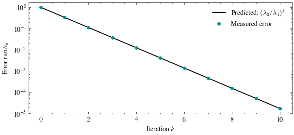
Predict before you plot. Lecture showed that each multiplication shrinks the unwanted \(\mathbf{v}_2\)-component by the factor \(\lambda_2/\lambda_1 = \frac13\) relative to the \(\mathbf{v}_1\)-component. So on a log-scale plot, the error should fall on a straight line, dropping by a factor of \(3\) every iteration. As in lecture, measure the error by \(\tan\theta_k\): the size of the component perpendicular to \(\mathbf{v}_1\) divided by the size of the component along it.

ks = np.arange(len(iterates))
errors = [abs(np.dot(vk, v2)) / abs(np.dot(vk, v1)) for vk in iterates]

fig, ax = plt.subplots(figsize=(7, 3))
ax.semilogy(ks, (1 / 3.0) ** ks, color="black", linewidth=1.3,
            label=r"Predicted: $(\lambda_2/\lambda_1)^k$")
ax.semilogy(ks, errors, "o", color=TEAL, markersize=4, label="Measured error")
ax.set_xlabel("Iteration $k$")
ax.set_xticks(range(0, 11, 2))
ax.set_ylabel(r"Error $\tan\theta_k$")
ax.legend(frameon=False)
plt.show()

The dots land on the predicted line, so the slope was knowable before we ran a single iteration.

What if the eigenvalues are close?

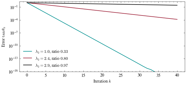
The prediction says the ratio \(\lambda_2/\lambda_1\) is everything. Keep the same eigenvectors but dial \(\lambda_2\) up toward \(\lambda_1 = 3\) by rebuilding \(\mathbf{A} = 3\,\mathbf{v}_1\mathbf{v}_1^\top + \lambda_2\,\mathbf{v}_2\mathbf{v}_2^\top\). Try your own \(\lambda_2\). How slow can you make it?

lambda2s = [1.0, 2.4, 2.9]   # change me! (keep below lambda1 = 3)
colors = [TEAL, CARDINAL, "black"]

fig, ax = plt.subplots(figsize=(7, 3))
for lam2, color in zip(lambda2s, colors):
    A2 = 3 * np.outer(v1, v1) + lam2 * np.outer(v2, v2)
    v = np.array([1.0, 0.0])
    errs = [1.0]
    for k in range(40):
        w = A2 @ v
        v = w / np.linalg.norm(w)
        errs.append(abs(np.dot(v, v2)) / abs(np.dot(v, v1)))
    ax.semilogy(errs, color=color, linewidth=1.3,
                label=rf"$\lambda_2 = {lam2}$, ratio ${lam2/3:.2f}$")
ax.set_xlabel("Iteration $k$")
ax.set_ylabel(r"Error $\tan\theta_k$")
ax.set_ylim(1e-16, 2)
ax.legend(frameon=False)
plt.show()

Punchline: the power method’s speed is set by the eigengap alone. Every iteration shrinks the error by the factor \(\lambda_2/\lambda_1\), so a runner-up eigenvalue close to the top costs us hundreds of iterations instead of a dozen. Problem 4 turns the slope you just saw into an exact iteration count for any accuracy \(\epsilon\).