Decompositions

Last lecture ended with a question. Every matrix we applied (the rotation, the scaling, the shear) warped the grid by rotating and stretching it, and we learned to read the warp from the columns: the columns are where the basis vectors land. But the basis vectors \(\mathbf{e}_1, \ldots, \mathbf{e}_d\) are our choice of directions, and a matrix has no reason to respect them. Today we ask for the directions the matrix itself prefers:

Which directions does a matrix merely stretch?

Chasing this question gives us eigenvectors, an algorithm for finding them, and, for matrices of any shape, the singular value decomposition, the most important factorization in this course. Today closes the Mathematical Foundations unit, and the rest of the semester leans on the SVD constantly: it will reappear when we fit linear models, when we compress data, and inside a modern optimizer for neural networks.

Eigenvalues and Eigenvectors

Consider a square matrix \(\mathbf{A} \in \mathbb{R}^{d \times d}\). An eigenvector of \(\mathbf{A}\) is a nonzero vector \(\mathbf{v} \in \mathbb{R}^d\) that the map does not rotate: \[ \mathbf{A}\mathbf{v} = \lambda \mathbf{v} \] for some scalar \(\lambda\), called the eigenvalue of \(\mathbf{v}\). On the line through \(\mathbf{v}\), the whole linear map collapses to ordinary multiplication: stretch by \(\lambda\) if \(\lambda > 1\), shrink if \(0 < \lambda < 1\), flip if \(\lambda < 0\).

Our running example for the day is a small symmetric matrix: \[ \mathbf{A} = \begin{bmatrix} 2 & 1 \\ 1 & 2 \end{bmatrix}. \] Two directions pass the eigenvector test, and both are cheap to check by hand: \[ \mathbf{A}\begin{bmatrix} 1 \\ 1 \end{bmatrix} = \begin{bmatrix} 2 + 1 \\ 1 + 2 \end{bmatrix} = 3\begin{bmatrix} 1 \\ 1 \end{bmatrix}, \qquad \mathbf{A}\begin{bmatrix} 1 \\ -1 \end{bmatrix} = \begin{bmatrix} 2 - 1 \\ 1 - 2 \end{bmatrix} = 1 \cdot \begin{bmatrix} 1 \\ -1 \end{bmatrix}. \] The first direction comes back pointing the same way and three times longer; the second comes back untouched. Eigenvectors carry a direction and not a length, since scaling \(\mathbf{v}\) scales both sides of \(\mathbf{A}\mathbf{v} = \lambda\mathbf{v}\) equally, so we normalize them and record the pair: \[ \mathbf{v}_1 = \tfrac{1}{\sqrt{2}}\begin{bmatrix} 1 \\ 1 \end{bmatrix} \text{ with } \lambda_1 = 3, \qquad \mathbf{v}_2 = \tfrac{1}{\sqrt{2}}\begin{bmatrix} 1 \\ -1 \end{bmatrix} \text{ with } \lambda_2 = 1. \] Every other direction in the plane gets rotated at least a little; these two are only stretched. (Not every matrix has such a direction. Can you see why last lecture’s rotation \(\mathbf{A}^{\mathrm{rot}}\) has no real eigenvector at all, unless \(\theta\) is a multiple of \(180^\circ\)?)

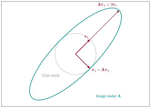
In the plot, \(\mathbf{A}\) maps the gray unit circle to the teal ellipse. The two cardinal arrows are the eigenvectors, the only directions whose image stays on its own line: \(\mathbf{v}_1\) is carried out to the dashed arrow at \(3\mathbf{v}_1\), while \(\mathbf{v}_2\) does not move. The eigenvectors are the ellipse’s axes, and the axes are perpendicular because \(\mathbf{A}\) is symmetric.

The Spectral Theorem

For symmetric matrices (\(\mathbf{A}^\top = \mathbf{A}\)), the eigenvectors do everything we could ask of a coordinate system. The spectral theorem says that every symmetric \(\mathbf{A} \in \mathbb{R}^{d \times d}\) has \(d\) real eigenvalues \(\lambda_1 \geq \lambda_2 \geq \cdots \geq \lambda_d\) and an orthonormal basis of eigenvectors \(\mathbf{v}_1, \ldots, \mathbf{v}_d\): each has unit length and any two are orthogonal. We will not prove the whole theorem, but the orthogonality half is a three-line argument: compute \(\lambda_i \langle \mathbf{v}_i, \mathbf{v}_j \rangle\) two ways and let symmetry do the work.

Claim: If \(\mathbf{A}\) is symmetric and \(\mathbf{A}\mathbf{v}_i = \lambda_i \mathbf{v}_i\), \(\mathbf{A}\mathbf{v}_j = \lambda_j \mathbf{v}_j\) with \(\lambda_i \neq \lambda_j\), then \(\langle \mathbf{v}_i, \mathbf{v}_j \rangle = 0\).

Proof of Claim

We compute the same number two ways: \[ \lambda_i \langle \mathbf{v}_i, \mathbf{v}_j \rangle = (\mathbf{A}\mathbf{v}_i)^\top \mathbf{v}_j = \mathbf{v}_i^\top \mathbf{A}^\top \mathbf{v}_j = \mathbf{v}_i^\top \mathbf{A} \mathbf{v}_j = \lambda_j \langle \mathbf{v}_i, \mathbf{v}_j \rangle. \] Here, we used that transposing a product reverses its order, and then symmetry to replace \(\mathbf{A}^\top\) with \(\mathbf{A}\). Subtracting, \((\lambda_i - \lambda_j)\langle \mathbf{v}_i, \mathbf{v}_j \rangle = 0\), and since \(\lambda_i \neq \lambda_j\), the inner product must vanish.

Collect the eigenvectors as the columns of \(\mathbf{V} \in \mathbb{R}^{d \times d}\) and the eigenvalues into the diagonal matrix \(\mathbf{\Lambda} = \mathrm{diag}(\lambda_1, \ldots, \lambda_d) \in \mathbb{R}^{d \times d}\). Then the whole matrix factors as the eigendecomposition: \[ \mathbf{A} = \mathbf{V} \mathbf{\Lambda} \mathbf{V}^\top = \sum_{i=1}^d \lambda_i \mathbf{v}_i \mathbf{v}_i^\top, \] where the second form is the outer-product view of matrix multiplication from last lecture, the matrix as a sum of rank-\(1\) pieces, one per eigenvector. Let’s sanity-check the sum by applying it to an eigenvector \(\mathbf{v}_j\): \[ \Big( \sum_{i=1}^d \lambda_i \mathbf{v}_i \mathbf{v}_i^\top \Big) \mathbf{v}_j = \sum_{i=1}^d \lambda_i \mathbf{v}_i \langle \mathbf{v}_i, \mathbf{v}_j \rangle = \lambda_j \mathbf{v}_j, \] where we pulled the scalar \(\mathbf{v}_i^\top \mathbf{v}_j = \langle \mathbf{v}_i, \mathbf{v}_j\rangle\) out of each outer product and used orthonormality: that inner product is \(0\) unless \(i = j\). This move, orthonormality collapses the sum, is the workhorse of today’s lecture.

Each term \(\lambda_i \mathbf{v}_i \mathbf{v}_i^\top\) acts only on the \(\mathbf{v}_i\) direction, so a symmetric matrix is \(d\) independent stretches in \(d\) perpendicular directions, and the numbers \(\lambda_i\) say how hard each one pulls. In the factored form, since \(\mathbf{V}\) is orthogonal (orthonormal columns, so \(\mathbf{V}^\top = \mathbf{V}^{-1}\) preserves lengths and angles), applying \(\mathbf{A}\) means: rotate the eigenbasis onto the coordinate axes (\(\mathbf{V}^\top\)), stretch each axis by its eigenvalue (\(\mathbf{\Lambda}\)), and rotate back (\(\mathbf{V}\)). Every symmetric matrix is just a stretch, viewed in the right coordinates.

Reading two eigenvectors off a \(2 \times 2\) matrix took one line of arithmetic. The theorem promises the same basis exists for a matrix with a million rows, but it says nothing about how to find a single one of them.

The Power Method

The matrices of this course have thousands or millions of rows, and we usually want only the top eigenvector, the direction of largest stretch. Finding it should be much cheaper than finding all \(d\), and it is.

The power method finds it with a single move applied over and over: multiply, normalize, repeat. Starting from a random unit vector \(\mathbf{v}^{(0)} \in \mathbb{R}^d\), iterate: \[ \mathbf{v}^{(k)} = \frac{\mathbf{A}\mathbf{v}^{(k-1)}}{\|\mathbf{A}\mathbf{v}^{(k-1)}\|_2}. \] The mechanical reason to expect this to work is the ellipse in the first figure. Multiplying by \(\mathbf{A}\) pulls hardest along \(\mathbf{v}_1\), so it tips whatever vector we are holding a little further toward \(\mathbf{v}_1\), and dividing by the norm keeps the vector on the unit circle instead of letting it run off to infinity.

The in-class exercise runs two iterations on our running example starting from \(\mathbf{v}^{(0)} = (1, 0)\). First iteration: \(\mathbf{A}\mathbf{v}^{(0)} = (2, 1)\), which normalizes to \(\mathbf{v}^{(1)} = \frac{1}{\sqrt{5}}(2, 1) \approx (0.894, 0.447)\). Second iteration: \(\mathbf{A}\mathbf{v}^{(1)} \propto (5, 4)\), which normalizes to \(\mathbf{v}^{(2)} = \frac{1}{\sqrt{41}}(5, 4) \approx (0.781, 0.625)\). Two matrix multiplications in, and we are visibly swinging toward the top eigenvector \(\mathbf{v}_1 \approx (0.707, 0.707)\).

Why does this work? Normalization only fixes the length, so the direction of \(\mathbf{v}^{(k)}\) is the direction of \(\mathbf{A}^k \mathbf{v}^{(0)}\), and powers of \(\mathbf{A}\) are easy to understand in the eigenbasis. Expand the start vector in the eigenvectors: \[ \mathbf{v}^{(0)} = \sum_{i=1}^d c_i \mathbf{v}_i, \qquad c_i = \langle \mathbf{v}_i, \mathbf{v}^{(0)} \rangle . \] Applying \(\mathbf{A}\) once shows what one step does to those coefficients: \[ \mathbf{A}\mathbf{v}^{(0)} = \mathbf{A}\sum_{i=1}^d c_i \mathbf{v}_i = \sum_{i=1}^d c_i \, \mathbf{A}\mathbf{v}_i = \sum_{i=1}^d \lambda_i c_i \, \mathbf{v}_i, \] where the second equality is linearity of the map and the third is the eigenvector equation applied one term at a time. Only the coefficients changed, so repeating the step \(k\) times gives: \[ \mathbf{A}^k \mathbf{v}^{(0)} = \sum_{i=1}^d \lambda_i^k c_i \mathbf{v}_i = \lambda_1^k \Big( c_1 \mathbf{v}_1 + \sum_{i=2}^d \Big(\frac{\lambda_i}{\lambda_1}\Big)^k c_i \mathbf{v}_i \Big), \] where the second equality pulled the largest eigenvalue out of every term. Every coefficient except the first is crushed by the factor \((\lambda_i / \lambda_1)^k \leq (\lambda_2/\lambda_1)^k\), so the direction converges to \(\mathbf{v}_1\), and the ratio \(\lambda_2 / \lambda_1\) sets the speed. The rate depends on one number, the gap between the top two eigenvalues, and it is slow exactly when the runner-up stretches almost as hard as the winner.

To turn “converges” into a number we can plot, let \(\theta_k\) be the angle between \(\mathbf{A}^k\mathbf{v}^{(0)}\) and the eigenvector \(\mathbf{v}_1\), and measure the error by \(\tan \theta_k\), the length of the part perpendicular to \(\mathbf{v}_1\) divided by the length of the part along it. In the running example, \(\mathbf{v}^{(0)} = (1,0) = \frac{1}{\sqrt{2}}(\mathbf{v}_1 + \mathbf{v}_2)\), so the two coefficients start out equal (\(\tan\theta_0 = 1\)) and after \(k\) steps the unwanted \(\mathbf{v}_2\)-component is \(3^{-k}\) times the size of the \(\mathbf{v}_1\)-component. Check it at \(k = 2\): the hand computation gave the direction \((5, 4) = \frac{1}{\sqrt 2}\left(9 \mathbf{v}_1 + \mathbf{v}_2\right)\), so \(\tan\theta_2 = 1/9 = 3^{-2}\). (One practical caveat: the argument needs \(c_1 \neq 0\), but a random starting vector satisfies this with probability \(1\).)

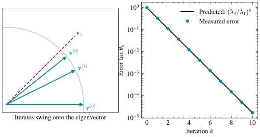
In the plot, the left panel shows the iterates swinging onto the eigenvector ray, and the right panel shows \(\tan\theta_k\) falling on a log scale: a straight line of slope \(\log(\lambda_2/\lambda_1) = \log(1/3)\) per iteration, exactly the crushing factor in the sum. Problem 4 turns this picture into an iteration count: about \(\log(1/\epsilon) / \log(\lambda_1/\lambda_2)\) steps are enough for accuracy \(\epsilon\), so the eigengap is the algorithm’s clock speed.

The method is cheap per step. Each iteration is one matrix–vector product, \(O(d^2)\) time, against \(O(d^3)\) to compute a full eigendecomposition, so it wins whenever we want one eigenvector of a large matrix rather than all of them. (Google’s original PageRank algorithm ranked the web by running the power method on a sparse matrix with billions of rows; a few dozen iterations sufficed.)

Every matrix in this section has been square. Our data will not be.

The Singular Value Decomposition

A data matrix \(\mathbf{A} \in \mathbb{R}^{n \times d}\) holding \(n\) points with \(d\) features almost never has \(n = d\), and for such a matrix the equation \(\mathbf{A}\mathbf{v} = \lambda \mathbf{v}\) does not even typecheck: the input lives in \(\mathbb{R}^d\) and the output in \(\mathbb{R}^n\), so they cannot be multiples of each other. A version of the story survives anyway, for every matrix, once we stop insisting that the input and output directions be the same and allow a different orthonormal basis on each side.

The singular value decomposition (SVD) of a matrix \(\mathbf{A} \in \mathbb{R}^{n \times d}\) of rank \(r\) is: \[ \mathbf{A} = \mathbf{U} \mathbf{\Sigma} \mathbf{V}^\top = \sum_{i=1}^r \sigma_i \mathbf{u}_i \mathbf{v}_i^\top, \] where the singular values \(\sigma_1 \geq \sigma_2 \geq \cdots \geq \sigma_r > 0\) are positive scalars, the left singular vectors \(\mathbf{u}_1, \ldots, \mathbf{u}_r \in \mathbb{R}^n\) are orthonormal, and the right singular vectors \(\mathbf{v}_1, \ldots, \mathbf{v}_r \in \mathbb{R}^d\) are orthonormal. In factored form, \(\mathbf{U} \in \mathbb{R}^{n \times r}\) and \(\mathbf{V} \in \mathbb{R}^{d \times r}\) collect the singular vectors as columns and \(\mathbf{\Sigma} = \mathrm{diag}(\sigma_1, \ldots, \sigma_r) \in \mathbb{R}^{r \times r}\). Every matrix has one, square or not, symmetric or not, full rank or not.

The decomposition says the map routes each right singular vector to its left partner, which we can see by collapsing the sum exactly as we did for the eigendecomposition: \[ \mathbf{A}\mathbf{v}_j = \Big( \sum_{i=1}^r \sigma_i \mathbf{u}_i \mathbf{v}_i^\top \Big) \mathbf{v}_j = \sum_{i=1}^r \sigma_i \mathbf{u}_i \langle \mathbf{v}_i, \mathbf{v}_j \rangle = \sigma_j \mathbf{u}_j . \] Geometrically, \(\mathbf{V}^\top\) rotates the input so the right singular vectors align with the axes, \(\mathbf{\Sigma}\) stretches axis \(i\) by \(\sigma_i\), and \(\mathbf{U}\) rotates the result into the output space:

every matrix is a rotation, then a stretch, then a rotation.

That claim should bother you, because last lecture’s shear seems to slide the plane sideways rather than stretch it along any axis. The SVD says otherwise.

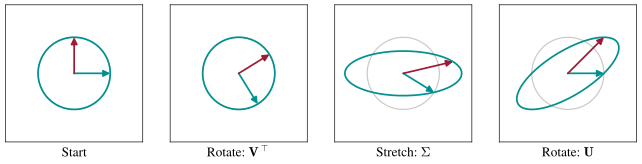
In the plot, the shear \(\mathbf{A}^{\mathrm{shear}} = \begin{bmatrix} 1 & 1 \\ 0 & 1 \end{bmatrix}\) is decomposed into its three SVD factors acting on the unit circle: a rotation, then a stretch along the axes, then another rotation, landing exactly on the shear’s tilted ellipse. The sliding is what the rotations look like once the stretching is done.

Where do singular values come from, and how do they relate to eigenvalues? The idea is that multiplying \(\mathbf{A}\) by its own transpose squares each stretch and cancels the rotations, which should leave a symmetric matrix we already know how to read. Multiply \(\mathbf{A}^\top \mathbf{A}\) using the outer-product form and collapse: \[ \mathbf{A}^\top \mathbf{A} = \Big( \sum_{i=1}^r \sigma_i \mathbf{v}_i \mathbf{u}_i^\top \Big) \Big( \sum_{j=1}^r \sigma_j \mathbf{u}_j \mathbf{v}_j^\top \Big) = \sum_{i=1}^r \sum_{j=1}^r \sigma_i \sigma_j \mathbf{v}_i \langle \mathbf{u}_i, \mathbf{u}_j \rangle \mathbf{v}_j^\top = \sum_{i=1}^r \sigma_i^2 \mathbf{v}_i \mathbf{v}_i^\top, \] where transposing reversed each outer product and orthonormality of the \(\mathbf{u}_i\) killed every cross term. But the right-hand side is an eigendecomposition! \(\mathbf{A}^\top \mathbf{A}\) is symmetric, its eigenvectors are the right singular vectors of \(\mathbf{A}\), and its eigenvalues are the squared singular values \(\sigma_i^2\). (The same argument on \(\mathbf{A}\mathbf{A}^\top\) produces the left singular vectors, and applying the spectral theorem to \(\mathbf{A}^\top\mathbf{A}\) is how the SVD is proved to exist.) The link also tells us how to read the largest singular value: it is the most that \(\mathbf{A}\) can stretch any unit vector, since \(\|\mathbf{A}\mathbf{v}_1\|_2 = \sigma_1\) and any other unit vector mixes in smaller singular values. And it says how to find the top one: run the power method on \(\mathbf{A}^\top\mathbf{A}\), which never requires forming that matrix, since each iteration can multiply by \(\mathbf{A}\) and then by \(\mathbf{A}^\top\).

The second in-class exercise verifies this on the running example. For \(\mathbf{A} = \begin{bmatrix} 2 & 1 \\ 1 & 2 \end{bmatrix}\), the product is symmetric, as promised: \[ \mathbf{A}^\top \mathbf{A} = \begin{bmatrix} 2 & 1 \\ 1 & 2 \end{bmatrix}\begin{bmatrix} 2 & 1 \\ 1 & 2 \end{bmatrix} = \begin{bmatrix} 5 & 4 \\ 4 & 5 \end{bmatrix}, \] whose eigenvectors are again \((1,1)/\sqrt 2\) and \((1,-1)/\sqrt 2\), now with eigenvalues \(9\) and \(1\). Taking square roots, the singular values are \(\sigma_1 = 3\) and \(\sigma_2 = 1\), matching the eigenvalues we started with. For a symmetric matrix whose eigenvalues are all nonnegative, the SVD is the eigendecomposition. (When a symmetric matrix has a negative eigenvalue \(\lambda\), the singular value is \(|\lambda|\): the stretch factor is a magnitude, and the sign hides in the rotations.) Squaring is what let us read the singular values off \(\mathbf{A}^\top\mathbf{A}\), and it is also what makes that matrix a risky thing to hand a computer, since the ratio of the largest singular value to the smallest gets squared along with them. The Optimization lecture will give that ratio a name, the condition number, and blame it for everything slow or fragile about fitting a linear model.

Looking Forward

The Mathematical Foundations unit is complete: probability gave us a language for uncertainty and the Monte Carlo estimator, and linear algebra closes with the decompositions that say what a map really does.

We front-loaded the SVD because the course uses it everywhere. When we fit our first model in the next unit, the SVD will solve least squares and explain when the solution is numerically fragile. In the Low-Rank Structure unit, keeping only the largest \(\sigma_i \mathbf{u}_i \mathbf{v}_i^\top\) terms will turn out to be the best way to compress a matrix, which is what makes image compression, embeddings, and efficient finetuning work. And near the end, an optimizer called Muon will improve neural network training by editing the singular values of the gradient itself.

Next lecture, the machine learning begins: what does it mean to learn a function from examples, and what should we ask of a good prediction? The answer starts, as so much of this course does, with probability.

Carry one sentence out of today: every matrix, viewed in the right orthonormal directions on each side, does nothing but stretch each direction by its own number, and most of the algorithms in this course are ways of getting at those numbers efficiently.