Demo: Loading Data, One Batch at a Time

The data we have modeled so far has been synthetic: thirty ice-cream days we generated ourselves. Real datasets are bigger, messier, and usually too large to look at all at once. Today we load a real one, California census blocks, with features like median income and a label of median house value.

import numpy as np
import matplotlib.pyplot as plt
import scienceplots
from sklearn.datasets import fetch_california_housing

plt.style.use(["science", "no-latex"])
TEAL, CARDINAL, GRAY = "#009090", "#9c1b33", "#c9c9c9"
rng = np.random.default_rng(6)

data = fetch_california_housing()
X, y = data.data, data.target
print("n, d =", X.shape)
print("features:", data.feature_names)
print("first row:", X[0])
print("first label (median house value, $100k):", y[0])

n, d = (20640, 8)
features: ['MedInc', 'HouseAge', 'AveRooms', 'AveBedrms', 'Population', 'AveOccup', 'Latitude', 'Longitude']
first row: [   8.3252       41.            6.98412698    1.02380952  322.
    2.55555556   37.88       -122.23      ]
first label (median house value, $100k): 4.526

The feature we’ll watch is MedInc, median income in tens of thousands of dollars. Its mean over all \(n = 20{,}640\) blocks is a fixed number. But if we only ever see a random batch \(S\), what do we see instead?

medinc = X[:, data.feature_names.index("MedInc")]
true_mean = medinc.mean()
print(f"true mean over all n = {len(medinc)} blocks: {true_mean:.2f}")

for batch_size in [10, 200]:
    batch = rng.choice(medinc, size=batch_size, replace=False)
    print(f"one random batch, |S| = {batch_size:3d}: batch mean = {batch.mean():.2f}")

true mean over all n = 20640 blocks: 3.87
one random batch, |S| =  10: batch mean = 5.13
one random batch, |S| = 200: batch mean = 3.99

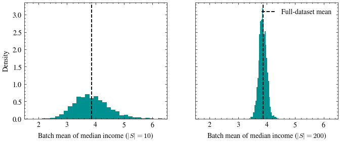
One batch is noisy, and a small batch is noisier than a big one. Let’s see the whole distribution: draw many random batches of each size and histogram their means, exactly like the dice histograms from Unit 1.

def batch_means(batch_size, n_batches=2000):
    return np.array([rng.choice(medinc, size=batch_size, replace=False).mean()
                      for _ in range(n_batches)])

fig, axes = plt.subplots(1, 2, figsize=(8, 3), sharey=True)
for ax, batch_size in zip(axes, [10, 200]):
    means = batch_means(batch_size)
    ax.hist(means, bins=30, color=TEAL, density=True)
    ax.axvline(true_mean, color="black", linestyle="--", linewidth=1.3, label="Full-dataset mean")
    ax.set_xlabel(f"Batch mean of median income ($|S| = {batch_size}$)")
    ax.set_xlim(1.5, 6.5)
axes[0].set_ylabel("Density")
axes[1].legend(frameon=False, loc="upper right")
plt.show()

This is Unit 1’s \(\sigma/\sqrt{n}\) rate, where \(\sigma\) is now the spread of median income across blocks. A batch mean is the sample mean of a random subset, so its spread shrinks like \(1/\sqrt{|S|}\). Let’s check that against the numbers.

sigma = medinc.std()
for batch_size in [10, 50, 200, 1000]:
    measured = batch_means(batch_size, n_batches=500).std()
    predicted = sigma / np.sqrt(batch_size)
    print(f"|S| = {batch_size:4d}   measured std = {measured:.3f}   predicted sigma/sqrt(|S|) = {predicted:.3f}")

|S| =   10   measured std = 0.618   predicted sigma/sqrt(|S|) = 0.601
|S| =   50   measured std = 0.271   predicted sigma/sqrt(|S|) = 0.269
|S| =  200   measured std = 0.132   predicted sigma/sqrt(|S|) = 0.134
|S| = 1000   measured std = 0.060   predicted sigma/sqrt(|S|) = 0.060

What if we shrank the batch further?

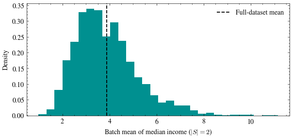
Try batch_size = 2 below. A batch this small barely deserves the word “average,” and the histogram shows why.

batch_size = 2    # change me!

means = batch_means(batch_size, n_batches=2000)
fig, ax = plt.subplots(figsize=(7, 3))
ax.hist(means, bins=30, color=TEAL, density=True)
ax.axvline(true_mean, color="black", linestyle="--", linewidth=1.3, label="Full-dataset mean")
ax.set_xlabel(f"Batch mean of median income ($|S| = {batch_size}$)")
ax.set_ylabel("Density")
ax.legend(frameon=False)
plt.show()
print(f"measured std = {means.std():.3f}   predicted = {sigma / np.sqrt(batch_size):.3f}")

measured std = 1.338   predicted = 1.343

Punchline: a batch is a sample, so every batch statistic is a noisy but unbiased stand-in for the full-dataset quantity, and its noise shrinks exactly like Unit 1 predicts. That is why the batch loss \(\mathcal{L}_S(f)\) we defined today can replace the full mean squared error \(\mathcal{L}(f)\) during training: same target, \(1/\sqrt{|S|}\) noise, a fraction of the work. Next lecture picks the model class \(f\) comes from.