Mean Squared Error
Last lecture we set the target \(f^*(x) = \mathbb{E}[Y \mid X = x]\) and then picked a hypothesis by instinct, scoring each candidate curve in the demo by its sum of squared gaps.
Today we stop guessing and derive. We will write down the probability that a hypothesis assigns to the data we actually saw, and ask which hypothesis makes that probability largest.
To write down a probability at all, we have to commit to a distribution for the noise, and the loss that falls out is a record of which distribution we committed to. Change the noise model and the loss changes with it.
Likelihood Under Gaussian Noise
Recall the noise model from last lecture: \[ y = f(\mathbf{x}) + \eta, \qquad \mathbb{E}[\eta] = 0, \] where \(f\) is a candidate hypothesis, \(\mathbf{x} \in \mathbb{R}^d\) is a feature vector, and the noise \(\eta \in \mathbb{R}\) collects everything about the label our features cannot see. Knowing that the noise averages to zero is not enough to compute a likelihood, so we commit to the distribution the Probability lecture singled out for exactly this purpose, the Gaussian: \[ \eta \sim \mathcal{N}(0, \sigma^2), \] where the noise level \(\sigma^2 > 0\) is the variance of the noise, one number shared by every data point. The justification is the one the Probability lecture gave: measurement noise is usually the sum of many small independent effects, and such sums pile up into a bell curve.
Fix a hypothesis \(f\) and a feature vector \(\mathbf{x}\). Under \(f\) the label is the prediction plus Gaussian noise, so the label itself is Gaussian, centered at the prediction: \[ y \mid \mathbf{x} \sim \mathcal{N}\big(f(\mathbf{x}), \sigma^2\big). \] Writing out the Gaussian density from Unit 1 gives the density that hypothesis \(f\) assigns to seeing the label \(y\) at features \(\mathbf{x}\): \[ p_f(y \mid \mathbf{x}) = \frac{1}{\sqrt{2\pi\sigma^2}} \exp\left(-\frac{(y - f(\mathbf{x}))^2}{2\sigma^2}\right). \] (The label is continuous, so this is a density rather than a probability; nothing below turns on the difference.)
It is largest when the prediction lands exactly on the label, and it falls off as the prediction moves away at a rate set by \(\sigma^2\): when \(\sigma^2\) is small a miss of two cones is already implausible, and when \(\sigma^2\) is large the same miss is unremarkable. Inside the exponent, the squared gap between label and prediction is already here, before we have said a word about loss functions. For now, treat \(\sigma^2\) as fixed and known (the Methodology lecture asks what happens when we have to estimate it too). That is one data point, and a dataset is many, so the next step is to score a hypothesis on all of them at once.
A Two-Point Warm-Up
Before turning the crank in general, let’s see the idea on two data points, exactly as we will do live in class. The gap between a label and its prediction shows up in every line from here on, so give it a name. Define the residual of hypothesis \(f\) on data point \(i\): \[ r^{(i)} = y^{(i)} - f(\mathbf{x}^{(i)}) \in \mathbb{R}, \] positive when the hypothesis predicts too low and negative when it predicts too high.
Suppose a hypothesis \(f\) predicts \(40\) cones on a mild day and \(55\) cones on a hot day, and nature delivers \(y^{(1)} = 42\) and \(y^{(2)} = 53\), so \(r^{(1)} = 2\) and \(r^{(2)} = -2\). The two days are independent (one customer’s cone doesn’t cause another’s), so the joint density of the two labels is the product of the two individual densities: \[ L(f) = \underbrace{\frac{1}{\sqrt{2\pi\sigma^2}}\exp\left(-\frac{(r^{(1)})^2}{2\sigma^2}\right)}_{\text{day 1}} \cdot \underbrace{\frac{1}{\sqrt{2\pi\sigma^2}}\exp\left(-\frac{(r^{(2)})^2}{2\sigma^2}\right)}_{\text{day 2}}. \] Products of exponentials are awkward to compare and logarithms turn products into sums, so we work with the log-likelihood: \[ \ell(f) = \log L(f). \] Taking that logarithm, one move per line: \[ \begin{align*} \ell(f) &= \log\left[\frac{1}{\sqrt{2\pi\sigma^2}}\exp\left(-\frac{(r^{(1)})^2}{2\sigma^2}\right)\right] + \log\left[\frac{1}{\sqrt{2\pi\sigma^2}}\exp\left(-\frac{(r^{(2)})^2}{2\sigma^2}\right)\right] \\&= -\frac{1}{2}\log(2\pi\sigma^2) - \frac{(r^{(1)})^2}{2\sigma^2} - \frac{1}{2}\log(2\pi\sigma^2) - \frac{(r^{(2)})^2}{2\sigma^2} \\&= -\log(2\pi\sigma^2) - \frac{(r^{(1)})^2 + (r^{(2)})^2}{2\sigma^2} . \end{align*} \] The first equality is the log of a product. The second applies \(\log \exp(u) = u\) and \(\log (2\pi\sigma^2)^{-1/2} = -\frac12\log(2\pi\sigma^2)\) inside each factor, and the third collects the two identical constants.
Two things to notice, both of which survive to the general case. First, the log turned a product into a sum, with one term per data point. Second, the hypothesis enters only through its squared residuals; the constant \(-\log(2\pi\sigma^2)\) out front is the same number for every hypothesis with the same \(\sigma\). Can you already see which part of \(\ell\) a search over hypotheses is able to move?
From Likelihood to Mean Squared Error
Nothing in the warm-up used the number two: independence makes the joint density a product however many points there are, and the logarithm makes that product a sum with one term per point.
Take a dataset of \(n\) points, assumed independent. The likelihood of the whole dataset under \(f\) is a product of \(n\) densities: \[ L(f) = \prod_{i=1}^n \frac{1}{\sqrt{2\pi\sigma^2}} \exp\left(-\frac{(y^{(i)} - f(\mathbf{x}^{(i)}))^2}{2\sigma^2}\right), \] and maximum likelihood asks us to solve \(\max_f L(f)\). Taking logs and simplifying, one move per line: \[ \begin{align*} \arg\max_f L(f) &= \arg\max_f \log L(f) \\&= \arg\max_f \sum_{i=1}^n \left[ -\frac{1}{2}\log(2\pi\sigma^2) - \frac{(y^{(i)} - f(\mathbf{x}^{(i)}))^2}{2\sigma^2} \right] \\&= \arg\max_f \left[ -\frac{n}{2}\log(2\pi\sigma^2) - \frac{1}{2\sigma^2}\sum_{i=1}^n (y^{(i)} - f(\mathbf{x}^{(i)}))^2 \right] \\&= \arg\min_f \sum_{i=1}^n (y^{(i)} - f(\mathbf{x}^{(i)}))^2 \\&= \arg\min_f \frac{1}{n}\sum_{i=1}^n (y^{(i)} - f(\mathbf{x}^{(i)}))^2. \end{align*} \] The first two equalities are the warm-up’s log rules run for \(n\) points (the log is monotonically increasing, so it preserves the \(\arg\max\)); after that, the constant \(-\frac{n}{2}\log(2\pi\sigma^2)\) does not depend on \(f\), maximizing the negative of a quantity is minimizing the quantity, and scaling by the positive constants \(2\sigma^2\) and \(1/n\) leaves the minimizer where it is. The hypothesis that makes the data most likely under Gaussian noise is exactly the hypothesis that minimizes the average squared residual.
That average is the crude score from last lecture’s demo, and now it gets its name. The mean squared error of a hypothesis \(f\) is the average of its squared residuals over the dataset: \[ \mathcal{L}(f) = \frac{1}{n}\sum_{i=1}^n \big(y^{(i)} - f(\mathbf{x}^{(i)})\big)^2 = \frac{1}{n}\sum_{i=1}^n \big(r^{(i)}\big)^2 . \] It penalizes the size of a miss and not its direction, since squaring throws away the sign of \(r^{(i)}\). And it penalizes quadratically, so one residual of \(4\) costs as much as sixteen residuals of \(1\): the loss is dominated by the worst-fit points.
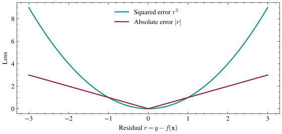
In the plot, both losses are drawn as functions of a single residual \(r = y - f(\mathbf{x})\): squared error \(r^2\) in teal and absolute error \(|r|\) in cardinal. Inside \(|r| < 1\) the parabola is the gentler of the two; past \(|r| = 1\) it pulls away, and at \(r = 3\) it penalizes three times what absolute error does. Absolute error comes back below, first as a loss with a different answer and then with a noise model of its own.
Choosing squared error as our loss and choosing Gaussian noise as our model of the world are the same decision, made once. That answers today’s question, and it leaves one loose thread: the noise level \(\sigma^2\) entered the likelihood and then dropped out of the \(\arg\min\), because a single shared \(\sigma^2\) only rescales the sum. We come back to it below, where it stops dropping out.
With a loss in hand, fitting a model turns into a search, and that search has a name.
Empirical Risk Minimization
Empirical risk minimization picks the hypothesis in a model class \(\mathcal{F}\) that minimizes a loss computed on the observed data: \[ \hat f = \arg\min_{f \in \mathcal{F}} \; \mathcal{L}(f) . \] Today \(\mathcal{L}\) is the mean squared error and \(\mathcal{F}\) is left unspecified; linear functions arrive next lecture. The loss is empirical because it averages over the \(n\) points we happened to collect rather than the population quantity \(\mathbb{E}[(Y - f(X))^2]\) that last lecture minimized: the same gap as between an estimator and the quantity it estimates.
In practice we rarely compute \(\mathcal{L}(f)\) over all \(n\) points at once, since datasets can be too large to hold in memory. Instead we draw a random batch of indices \(S \subseteq \{1, \ldots, n\}\), typically with \(|S|\) in the hundreds while \(n\) runs to millions, and compute the loss restricted to it: \[ \mathcal{L}_S(f) = \frac{1}{|S|}\sum_{i \in S} \big(y^{(i)} - f(\mathbf{x}^{(i)})\big)^2 . \] This is exactly the Monte Carlo estimator from Unit 1. Each term is one sampled value of the per-point loss and \(\mathcal{L}_S(f)\) is the sample mean of \(|S|\) of them, so everything we proved about sample means transfers: the batch loss is an unbiased estimate of the full-data loss, and its spread shrinks like \(1/\sqrt{|S|}\). The class demo loads California house prices, the course’s first real dataset, and watches a batch mean tighten toward the full-dataset mean at exactly that rate. The same guarantee covers \(\mathcal{L}_S(f)\) itself, which is why stochastic gradient descent, built entirely on batch losses, still finds its way to a good hypothesis later in the course.
Empirical risk minimization says what to minimize; it does not say what the minimizer looks like.
The Best Constant, Revisited
Let’s run empirical risk minimization on the simplest model class there is: constant functions \(f(\mathbf{x}) = c\), which ignore the features entirely. This is the sample analogue of Problem 5 Part A, which found \(c^* = \mathbb{E}[Y]\) at the population level; here the average runs over a finite dataset \(y^{(1)}, \ldots, y^{(n)}\).
Claim: Under mean squared error, the best constant prediction is the sample mean of the labels; under mean absolute error, it is the sample median.
Proof of Claim
For squared error, differentiate \(\mathcal{L}(c) = \frac1n\sum_{i=1}^n (c - y^{(i)})^2\) with respect to \(c\) and set the result to zero: \[ \frac{d\mathcal{L}}{dc} = \frac2n \sum_{i=1}^n (c - y^{(i)}) = 0 \quad\Longleftrightarrow\quad c = \frac1n\sum_{i=1}^n y^{(i)} = \bar y . \] The loss is convex in \(c\) (a sum of upward-facing bowls), so this critical point is the unique minimum.
For absolute error, \(\mathcal{L}(c) = \frac1n \sum_i |c - y^{(i)}|\) is not differentiable at the data points, but away from them each term contributes \(+\frac1n\) if its label sits below \(c\) and \(-\frac1n\) if it sits above: \[ \frac{d\mathcal{L}}{dc} = \frac1n\Big(\#\{i : y^{(i)} < c\} - \#\{i : y^{(i)} > c\}\Big). \] Moving \(c\) up past a data point moves that point from the second count into the first, so the derivative is negative while \(c\) sits below the median (more points above than below pull it up) and positive once \(c\) passes it. The minimum sits where the two counts balance, which is the sample median.The two answers differ for a mechanical reason, visible in the loss plot above. The derivative of squared error grows with the residual, so a distant point pulls on the solution harder than a nearby one and the balance point is where the distances cancel, which is the mean. The derivative of absolute error is \(\pm 1\) however far away the point is, so every point pulls with the same strength and the balance point is where the counts cancel, which is the median. That is also why the median is the more robust summary: moving a single label out to a million drags the mean with it and leaves the median alone. (Problem 5 Part D\(^\star\) is the population version of this second half; the kink in \(|r|\) at \(0\) is also one practical reason to prefer squared error when we plan to take gradients.)
Two losses, two different answers on the same data. So which one is right?
Choosing a Loss Is Choosing a Noise Model
Neither is right on its own, because a loss is not something the data hands us. We derived squared error by assuming Gaussian noise, and every other loss comes out of the same recipe run with a different distribution: choosing a loss function is choosing a noise model.
Take absolute error, whose best constant we just computed. For its negative log-likelihood to be a sum of terms \(|r^{(i)}|\), the noise density has to carry \(|\eta|\) in its exponent, which points at the Laplace distribution: \[ p(\eta) = \frac{1}{2b}\exp\left(-\frac{|\eta|}{b}\right), \] where the scale \(b > 0\) plays the role \(\sigma\) plays for the Gaussian. Laplace noise is more sharply peaked at zero and heavier in the tails than a Gaussian of the same spread, so it expects most points to sit nearly on the curve and is not shocked by the occasional wild one. Problem 6 runs today’s derivation with this density in place of the Gaussian and reads off the loss that falls out.
The same recipe picks up the loose thread from above: what if the noise level is not the same for every point? Some measurements are simply noisier than others, like a thermometer read by a distracted intern versus a calibrated sensor. If point \(i\) carries its own noise level \(\sigma_i^2\), the likelihood still factors into a product of Gaussians, but now the \(\sigma_i^2\) inside the exponents are not one shared constant we can divide away, so they cannot leave the \(\arg\min\) the way a single \(\sigma^2\) did. Problem 6 finds where they end up, and the answer tells us which points a fit should trust.
Looking Forward
We still lack a model class to minimize over; next lecture commits to the simplest interesting one, linear functions, with the weights, design matrix, and feature maps that let a “linear” model bend to curves.
The three-step recipe (write the likelihood, take a log, turn the \(\arg\max\) into an \(\arg\min\)) returns: it hands us cross-entropy in the logistic regression lecture, and the ridge penalty in the Generalization lecture, where the Gaussian sits on the weights instead of the noise.
Carry one sentence out of today: a loss function is a claim about how the world adds noise to our labels, so choose the loss whose claim matches the errors you expect.