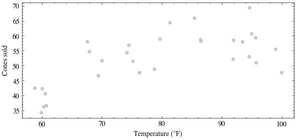
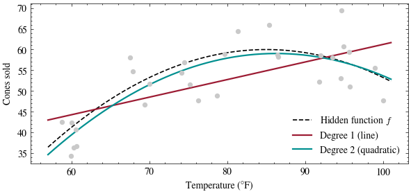
Last time we squinted at three candidate curves for the ice-cream scatter and eyeballed which one looked most plausible. Today we fit them for real, by handing a plain linear model a polynomial feature map \(\phi(t) = (1, t, t^2, \ldots, t^k)\) instead of just \(t\).
Build the design matrix by hand for a degree-\(k\) fit: one column per power of temperature. Then solve \(\mathbf{X}\mathbf{w} = \mathbf{y}\) in the least squares sense with np.linalg.lstsq. Next lecture derives that solver; today we just call it.
def design_matrix(t, degree):return np.column_stack([t ** k for k inrange(degree +1)])def fit(t, y, degree): X = design_matrix(t, degree) w, *_ = np.linalg.lstsq(X, y, rcond=None)return wdef predict(w, t): degree =len(w) -1return design_matrix(t, degree) @ wts = np.linspace(57, 101, 200)fig, ax = plt.subplots(figsize=(7, 3))ax.scatter(temps, sales, s=18, color=GRAY, zorder=3)ax.plot(ts, hidden_f(ts), color="black", linestyle="--", linewidth=1.2, label="Hidden function $f$")for degree, color, label in [(1, CARDINAL, "Degree 1 (line)"), (2, TEAL, "Degree 2 (quadratic)")]: w = fit(temps, sales, degree) ax.plot(ts, predict(w, ts), color=color, linewidth=1.6, label=label)print(f"degree {degree}: w = {np.round(w, 4)}")ax.set_xlabel("Temperature (°F)")ax.set_ylabel("Cones sold")ax.legend(frameon=False, loc="lower right")plt.show()
degree 1: w = [18.8568  0.4238]
degree 2: w = [-1.527021e+02  4.909900e+00 -2.850000e-02]
The degree-2 weights land near the hidden function’s own coefficients: expanding \(60 - 0.03(t - 85)^2\) gives \(-156.75 + 5.1t - 0.03t^2\). The model recovered a quadratic it was never told about, out of nothing but the features we handed it.
The reading’s other claim was geometric. Predictions \(\hat{\mathbf{y}} = \mathbf{X}\mathbf{w}\) live in the column space of \(\mathbf{X}\), and least squares picks the point of that subspace closest to \(\mathbf{y}\), so the residual \(\mathbf{r} = \mathbf{y} - \hat{\mathbf{y}}\) has to come out perpendicular to every column. Thirty points and three columns is more than we want to check by hand, so let’s check it in floating point.
X = design_matrix(temps, 2)w = fit(temps, sales, 2)r = sales - X @ wcosines = (X.T @ r) / (np.linalg.norm(X, axis=0) * np.linalg.norm(r))print("cosine of the angle between each column of X and the residual:")print(cosines)
cosine of the angle between each column of X and the residual:
[5.09728648e-12 5.42039652e-12 5.57966517e-12]
What if we kept adding degrees?
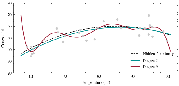
Push degree up and watch the fit start chasing individual days instead of the shared arc.
One practical note before we do. Raw powers of a temperature near \(100\) span many orders of magnitude, so the columns \(1, t, t^2, \ldots\) become hard to tell apart in floating point. Centering and scaling the input first fixes that: it changes the weights but not the fitted curve, and next lecture measures exactly this problem with the condition number.
Punchline: every curve here came from the same linear model and the same solver, and only the feature map changed. “Linear” describes the weights, never the shape of the curve. (Notice the high-degree fit threading individual days rather than the shared arc; telling those two apart is what the Methodology lecture is for.)