Linear Model
Two lectures ago we set the target, the regression function \(f^*(x) = \mathbb{E}[Y \mid X = x]\), the best predictor that could exist. Last lecture we derived the loss: mean squared error is what maximum likelihood hands back when we model the noise as Gaussian. Neither lecture picked what we search over: empirical risk minimization ranges over a model class \(\mathcal{F}\), and we have never said which functions are in it.
Today we commit to an answer: linear functions. The name promises straight lines, but with the right features a linear model draws a cubic; the restriction that is real has nothing to do with shape. Once the dataset is fixed, its predictions fill out only a \(d\)-dimensional slice of \(\mathbb{R}^n\), and fitting is nothing more than picking the point of that slice closest to the labels.
Weights, and a Bias
A linear model predicts a weighted sum of the features: \[ f(\mathbf{x}) = \langle \mathbf{w}, \mathbf{x}\rangle + b = \sum_{j=1}^d w_j x_j + b, \] where \(\mathbf{w} \in \mathbb{R}^d\) is a vector of weights, one per feature, and \(b \in \mathbb{R}\) is a single bias (or intercept). Each weight \(w_j\) says how much the prediction moves per unit change in feature \(j\), holding every other feature fixed, so a positive \(w_j\) for temperature means hotter days push sales up. That “holding every other feature fixed” is the model’s one substantive assumption about the world: feature \(j\) contributes \(w_j x_j\) whatever the other features are doing, so a linear model cannot express an interaction, like sales responding to heat only on weekends. The bias is what the model predicts when every feature is zero; without it, every hyperplane we could fit would be forced through the origin, which is rarely where the data actually sits.
A small trick removes the bias from the notation entirely. Append a constant feature equal to \(1\) to every \(\mathbf{x}\), and append \(b\) to the end of \(\mathbf{w}\): \[ \tilde{\mathbf{x}} = \begin{bmatrix} \mathbf{x} \\ 1 \end{bmatrix} \in \mathbb{R}^{d+1}, \qquad \tilde{\mathbf{w}} = \begin{bmatrix} \mathbf{w} \\ b \end{bmatrix} \in \mathbb{R}^{d+1}, \qquad\text{so that}\qquad \langle \tilde{\mathbf{w}}, \tilde{\mathbf{x}}\rangle = \langle \mathbf{w}, \mathbf{x}\rangle + b. \] From here on we drop the tildes and just write \(f(\mathbf{x}) = \langle \mathbf{w}, \mathbf{x}\rangle\), with the understanding that one entry of \(\mathbf{x}\) is a fixed \(1\) and the matching entry of \(\mathbf{w}\) is the bias. Every later lecture in this unit uses this convention, so the bias never needs its own symbol again. On the ice-cream data from the Regression lecture there is one raw feature, the temperature \(t\), so the model is a line \(f(t) = wt + b\) and the append trick gives it \(d = 2\) weights.
That is one prediction for one day, and our loss sums over all \(n\) of them.
The Design Matrix
Stack the \(n\) feature vectors into a matrix. The design matrix holds one data point per row, in the row notation from the Linear Algebra lecture: \[ \mathbf{X} \in \mathbb{R}^{n \times d}, \qquad [\mathbf{X}]_{i,} = (\mathbf{x}^{(i)})^\top . \] Because a matrix-vector product computes one inner product per row, stacking the predictions for all \(n\) points is a single matrix-vector product: \[ \hat{\mathbf{y}} = \mathbf{X}\mathbf{w} \in \mathbb{R}^n, \qquad \text{where } \hat{y}^{(i)} = \langle \mathbf{w}, \mathbf{x}^{(i)}\rangle. \] The prediction vector \(\hat{\mathbf{y}}\) has one entry per data point, so it sits in \(\mathbb{R}^n\) alongside the labels \(\mathbf{y}\), while the weights sit in \(\mathbb{R}^d\), one per feature. (Computing \(\hat{\mathbf{y}}\) costs \(O(nd)\), one multiply-add per entry of \(\mathbf{X}\).)
With both vectors in \(\mathbb{R}^n\), the mean squared error from last lecture collapses into a single norm: \[ \mathcal{L}(\mathbf{w}) = \frac1n \sum_{i=1}^n (y^{(i)} - \hat y^{(i)})^2 = \frac1n \|\mathbf{y} - \hat{\mathbf{y}}\|_2^2 = \frac1n \|\mathbf{y} - \mathbf{X}\mathbf{w}\|_2^2, \] where the first equality is the definition of the norm from the Linear Algebra lecture and the second substitutes \(\hat{\mathbf{y}} = \mathbf{X}\mathbf{w}\). The loss is the squared distance in \(\mathbb{R}^n\) between the label vector and the prediction vector, so fitting a linear model means sliding \(\hat{\mathbf{y}}\) as close to \(\mathbf{y}\) as the model allows.
Notice also that nothing in \(\mathcal{L}(\mathbf{w})\) depends on where the columns of \(\mathbf{X}\) came from; the design matrix is built once, from the data, before any fitting happens.
Feature Maps: Linear in the Parameters
A model that is linear in \(\mathbf{x}\) can only draw straight lines and flat hyperplanes, which rules out most of the datasets we care about. But fitting only ever required the prediction to be linear in \(\mathbf{w}\), and nothing stops us from filling the columns of \(\mathbf{X}\) with features that are themselves nonlinear functions of \(\mathbf{x}\).
A feature map transforms the raw input before the linear model ever sees it: \[ \phi: \mathbb{R}^d \to \mathbb{R}^{d'}, \qquad f(\mathbf{x}) = \langle \mathbf{w}, \phi(\mathbf{x})\rangle, \] where \(d'\) is the number of features after the map and \(\mathbf{w} \in \mathbb{R}^{d'}\) now carries one weight per transformed feature. The classic example is the polynomial basis. For a single input \(x\), take \(\phi(x) = (1, x, x^2, \ldots, x^{k}) \in \mathbb{R}^{k+1}\), and the prediction becomes a degree-\(k\) polynomial: \[ f(x) = w_0 + w_1 x + w_2 x^2 + \cdots + w_k x^k. \] This function curves and bends in \(x\) while staying linear in \(\mathbf{w}\), so every tool built for linear regression (today’s geometry, next lecture’s solvers) applies to it unchanged; only the design matrix’s columns change, from \(x^{(i)}\) itself to \(1, x^{(i)}, (x^{(i)})^2, \ldots\) (Polynomials are one choice among many. Sines and cosines give a Fourier basis, bumps centered at chosen points give a radial basis, and the fitting is the same for all of them.)
Let’s build one by hand, exactly as we will in class. Suppose we want a cubic passing exactly through four points: \((-1, 0)\), \((0, 0)\), \((1, 0)\), and \((2, 6)\). With four points and four weights (\(w_0, w_1, w_2, w_3\)), we expect a single hypothesis to fit exactly, so we can solve \(\mathbf{X}\mathbf{w} = \mathbf{y}\) directly rather than minimize anything. The design matrix stacks \(\phi(x^{(i)}) = (1, x^{(i)}, (x^{(i)})^2, (x^{(i)})^3)\) as rows: \[ \mathbf{X} = \begin{bmatrix} 1 & -1 & 1 & -1 \\ 1 & 0 & 0 & 0 \\ 1 & 1 & 1 & 1 \\ 1 & 2 & 4 & 8 \end{bmatrix}, \qquad \mathbf{y} = \begin{bmatrix} 0 \\ 0 \\ 0 \\ 6 \end{bmatrix}. \] Solve the four equations in order. The second row reads \(w_0 = 0\). Adding the first and third rows gives \(2w_0 + 2w_2 = 0\), so \(w_2 = 0\); subtracting the first from the third gives \(2w_1 + 2w_3 = 0\), so \(w_1 = -w_3\). The fourth row is then \(2w_1 + 8w_3 = 6\), and substituting \(w_1 = -w_3\) leaves \(6w_3 = 6\). So \(\mathbf{w} = (0, -1, 0, 1)^\top\), the fitted function is \(f(x) = x^3 - x\), and indeed \(f(-1) = f(0) = f(1) = 0\) while \(f(2) = 8 - 2 = 6\). Notice the model class never changed; we only changed what we handed it as “features.”
Four points fit exactly because we had exactly enough weights. With noisy data we go back to minimizing mean squared error, over the same expanded design matrix. The demo runs this fit on the ice-cream scatter from the Regression lecture and raises the degree from there, watching a line turn into a curve.
So shape is not where a linear model is limited. Where is it?
Predictions Live in the Column Space
The Linear Algebra lecture promised that the question “which predictions can our model even produce?” would turn out to be “what is the column space of the data matrix?” Expand the matrix-vector product \(\hat{\mathbf{y}} = \mathbf{X}\mathbf{w}\) one column at a time, the way that lecture taught us to read matrix multiplication: \[ \hat{\mathbf{y}} = \mathbf{X}\mathbf{w} = \sum_{j=1}^d w_j\, [\mathbf{X}]_{,j}, \] where \([\mathbf{X}]_{,j} \in \mathbb{R}^n\) is the \(j\)th column of \(\mathbf{X}\), holding the values of feature \(j\) across all \(n\) data points. By rows, \(\mathbf{X}\mathbf{w}\) says what the model predicts, one inner product per day; by columns it says what the model can predict, namely any mix of the \(d\) feature columns, with the weights supplying the amounts. Choosing \(\mathbf{w}\) chooses the amounts and nothing else, so \(\hat{\mathbf{y}}\) can never leave the column space of \(\mathbf{X}\): \[ \mathrm{col}(\mathbf{X}) = \{\mathbf{X}\mathbf{w} : \mathbf{w} \in \mathbb{R}^d\} \subseteq \mathbb{R}^n, \] a subspace whose dimension is the rank of \(\mathbf{X}\), at most \(d\). This is the restriction the opening warned about: \(\mathbf{y}\) is free to be any \(n\) numbers, while \(\hat{\mathbf{y}}\) is confined to \(d\) directions’ worth of them, however wildly the feature map bends the curve. In the cubic example above, \(n = d = 4\) and the four columns happened to span all of \(\mathbb{R}^4\), so an exact fit was possible. That is the exception, not the rule.
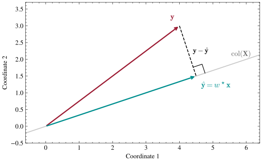
Consider the smallest case where the reach runs out: one feature (\(d=1\)) and two data points (\(n=2\)), so \(\mathrm{col}(\mathbf{X})\) is only a line through the origin in \(\mathbb{R}^2\). Take the single feature column \(\mathbf{x} = (3, 1)^\top\) and labels \(\mathbf{y} = (4, 3)^\top\). In the plot, \(\mathbf{y}\) sits off the line, so no scalar \(w\) satisfies \(w\mathbf{x} = \mathbf{y}\); an exact fit would need \(\mathbf{y}\) to be a multiple of \(\mathbf{x}\), and it is not. Minimizing is all we can do, and with a single weight we can do it by hand. Expand the squared distance, using that a squared norm is the inner product of a vector with itself: \[ \begin{align*} n\,\mathcal{L}(w) = \|\mathbf{y} - w\mathbf{x}\|_2^2 &= \langle \mathbf{y} - w\mathbf{x},\; \mathbf{y} - w\mathbf{x}\rangle \\&= \langle \mathbf{y}, \mathbf{y}\rangle - 2w\langle \mathbf{x}, \mathbf{y}\rangle + w^2 \langle \mathbf{x}, \mathbf{x}\rangle \\&= \|\mathbf{y}\|_2^2 - 2w\langle \mathbf{x}, \mathbf{y}\rangle + w^2\|\mathbf{x}\|_2^2 , \end{align*} \] where we foiled and used \(\langle \mathbf{x}, \mathbf{y}\rangle = \langle \mathbf{y}, \mathbf{x}\rangle\) to collect the cross terms. As a function of \(w\) this is an upward-facing parabola, so its one minimum is where the derivative vanishes: \[ \frac{d}{dw}\big(n\,\mathcal{L}(w)\big) = -2\langle \mathbf{x}, \mathbf{y}\rangle + 2w\|\mathbf{x}\|_2^2 = 0 \quad\Longleftrightarrow\quad w^\star = \frac{\langle \mathbf{x}, \mathbf{y}\rangle}{\|\mathbf{x}\|_2^2} . \] With \(\langle \mathbf{x}, \mathbf{y}\rangle = 3 \cdot 4 + 1 \cdot 3 = 15\) and \(\|\mathbf{x}\|_2^2 = 3^2 + 1^2 = 10\), the best weight is \(w^\star = 1.5\), the prediction is \(\hat{\mathbf{y}} = 1.5\,\mathbf{x} = (4.5, 1.5)^\top\), and the residual vector is \(\mathbf{r} = \mathbf{y} - \hat{\mathbf{y}} = (-0.5, 1.5)^\top\).
Now look at where that answer left the residual: \[ \langle \mathbf{x}, \mathbf{r}\rangle = \langle \mathbf{x}, \mathbf{y}\rangle - w^\star\|\mathbf{x}\|_2^2 = 15 - 1.5 \cdot 10 = 0 . \] Here the first equality expands \(\mathbf{r} = \mathbf{y} - w^\star\mathbf{x}\) by linearity, and the second substitutes the two numbers above. The residual is orthogonal to the feature column, which is the right angle drawn at the foot of the dashed line in the plot. The point \(\hat{\mathbf{y}}\) we landed on is called the projection of \(\mathbf{y}\) onto \(\mathrm{col}(\mathbf{X})\), and minimizing mean squared error is exactly the act of finding it: among all the vectors the model is capable of predicting, pick the one nearest to the labels we actually observed.
Perpendicularity is the mechanical reason that point is the closest one, and nothing about the reason depends on the dimension, so let’s prove it once for a design matrix of any size.
Claim: If \(\mathbf{w}^\star\) minimizes \(\|\mathbf{y} - \mathbf{X}\mathbf{w}\|_2^2\), then the residual \(\mathbf{r} = \mathbf{y} - \mathbf{X}\mathbf{w}^\star\) is orthogonal to every column of \(\mathbf{X}\).
Proof of Claim
Suppose not, so that \(\langle [\mathbf{X}]_{,j}, \mathbf{r}\rangle = c \neq 0\) for some column \(j\). Nudge that one weight, replacing \(\mathbf{w}^\star\) by \(\mathbf{w}^\star + \epsilon\mathbf{e}_j\) for a scalar \(\epsilon\), where \(\mathbf{e}_j\) is the \(j\)th basis vector. The prediction moves by \(\epsilon [\mathbf{X}]_{,j}\) and the residual becomes \(\mathbf{r} - \epsilon[\mathbf{X}]_{,j}\), so expanding the new squared distance exactly as in the one-column case gives: \[ \|\mathbf{r} - \epsilon[\mathbf{X}]_{,j}\|_2^2 = \|\mathbf{r}\|_2^2 - 2\epsilon c + \epsilon^2 \|[\mathbf{X}]_{,j}\|_2^2 . \] We get to pick \(\epsilon\), so pick the one that makes the change as negative as possible, \(\epsilon = c / \|[\mathbf{X}]_{,j}\|_2^2\): \[ \|\mathbf{r} - \epsilon[\mathbf{X}]_{,j}\|_2^2 = \|\mathbf{r}\|_2^2 - \frac{c^2}{\|[\mathbf{X}]_{,j}\|_2^2} < \|\mathbf{r}\|_2^2 . \] The nudge strictly lowered the loss, contradicting the assumption that \(\mathbf{w}^\star\) was a minimizer.As long as any of the miss still points along a feature, that feature has an improvement left in it; at the optimum, every feature has been used up.
One more thing is visible in the picture, and these numbers are small enough to check it. The prediction and the residual are perpendicular and add up to \(\mathbf{y}\), so they are the two legs of a right triangle whose hypotenuse is \(\mathbf{y}\): \[ \|\mathbf{y}\|_2^2 = 4^2 + 3^2 = 25, \qquad \|\hat{\mathbf{y}}\|_2^2 + \|\mathbf{r}\|_2^2 = (4.5^2 + 1.5^2) + (0.5^2 + 1.5^2) = 22.5 + 2.5 = 25 . \] The squared length of the labels splits cleanly into the part the model explains and the part it misses, with no cross term. Problem 7 asks you to prove that split in general, to turn the perpendicularity condition into an algebraic recipe for \(\mathbf{w}^\star\) (the normal equations), and to read the ratio of the two pieces as the goodness-of-fit score \(R^2\). Next lecture derives the same recipe from the other direction, by setting a gradient to zero, and the two answers had better agree.
Here is a question to leave open. What happens when \(d > n\), so the design matrix has more columns than rows? Then \(\mathrm{col}(\mathbf{X})\) can be all of \(\mathbb{R}^n\), every label vector is reachable, and infinitely many weight vectors fit the data exactly. The geometry stops helping at that point, because there is no longer a unique closest point to find. Which of those infinitely many exact fits should we prefer? The Generalization lecture at the end of the next unit needs an answer, and Problem 7 closes by pointing at the same gap.
Looking Forward
What we have not said is how to find the closest point when no exact fit exists. Next lecture answers that twice over, with an exact formula and an iterative alternative, and counts what each one costs in \(n\) and \(d\). It also reaches back to the SVD for the case where the columns of \(\mathbf{X}\) are nearly redundant, which our features invite: \(1, t, t^2, \ldots\) look more and more alike as the degree grows, and the condition number measures the damage.
Carry one sentence out of today: a model class is a set of reachable prediction vectors, not a set of shapes, and fitting picks the reachable one closest to the labels.