We have three ways to fit a linear model: the normal equations with an explicit inverse, the SVD-based pseudoinverse, and gradient descent. In exact arithmetic all three return the same \(\mathbf{w}^\star\). Today we watch what happens to each one when the design matrix is badly conditioned.
import numpy as npimport matplotlib.pyplot as pltimport scienceplotsplt.style.use(["science", "no-latex"])TEAL, CARDINAL, GRAY ="#009090", "#9c1b33", "#c9c9c9"rng = np.random.default_rng(8)n, d =200, 2w_true = np.array([2.0, -1.0])# feature 1 on a normal scale, feature 2 on a scale 1000x largerx1 = rng.normal(0, 1, size=n)x2 = rng.normal(0, 1, size=n) *1000X = np.column_stack([x1, x2])y = X @ w_true + rng.normal(0, 0.1, size=n)print("condition number of X: ", np.round(np.linalg.cond(X), 1))print("condition number of X^T X: ", np.round(np.linalg.cond(X.T @ X), 1))print("curvatures of the bowl: ", np.linalg.eigvalsh((2/ n) * X.T @ X))
condition number of X:      976.9
condition number of X^T X:  954332.3
curvatures of the bowl:     [2.16280813e+00 2.06403767e+06]
Squaring the condition number turned a large number into a much larger one, exactly as \(\kappa(\mathbf{X}^\top\mathbf{X}) = \kappa(\mathbf{X})^2\) says it must. The two curvatures \(\lambda_i = 2\sigma_i^2/n\) are the steep and shallow directions of the bowl, and their ratio is that same squared condition number. Now let’s fit with all three solvers.
The two closed-form solvers agree to every digit printed. A condition number of \(10^6\) on \(\mathbf{X}^\top\mathbf{X}\) is large, but not yet large enough to show up in double precision.
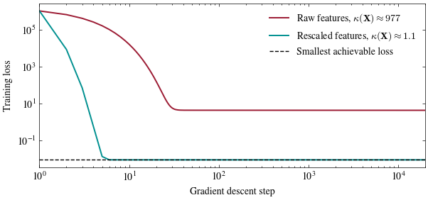
Gradient descent is another matter. After 20,000 steps it has the weight on the large-scale feature right to three decimals, while the other weight has crawled from its starting value of \(0\) to about \(0.009\) against a target of \(2.007\). That second weight is the shallow direction: with curvature \(2.2\) against \(2\times 10^6\), the step size that keeps the steep direction stable barely moves it at all.
def gd_loss_curve(X, y, alpha, steps): w = np.zeros(X.shape[1]) losses = []for _ inrange(steps): losses.append(np.mean((X @ w - y) **2)) w = w - alpha * (2/len(y)) * X.T @ (X @ w - y)return np.array(losses)# rescale each column to unit standard deviation: same column space, rounder bowlX_rescaled = X / X.std(axis=0)print("condition number after rescaling:", np.round(np.linalg.cond(X_rescaled), 2))steps =20000losses_raw = gd_loss_curve(X, y, alpha=1e-7, steps=steps)losses_rescaled = gd_loss_curve(X_rescaled, y, alpha=0.5, steps=steps)best = np.mean((X @ w_svd - y) **2)fig, ax = plt.subplots(figsize=(7, 3))ax.plot(np.arange(1, steps +1), losses_raw, color=CARDINAL, linewidth=1.4, label="Raw features, $\\kappa(\\mathbf{X}) \\approx 977$")ax.plot(np.arange(1, steps +1), losses_rescaled, color=TEAL, linewidth=1.4, label="Rescaled features, $\\kappa(\\mathbf{X}) \\approx 1.1$")ax.axhline(best, color="black", linestyle="--", linewidth=1.0, label="Smallest achievable loss")ax.set_xscale("log")ax.set_yscale("log")ax.set_xlim(1, steps)ax.set_xlabel("Gradient descent step")ax.set_ylabel("Training loss")ax.legend(frameon=False)plt.show()
condition number after rescaling: 1.09
Dividing each column by its standard deviation only rescales the columns, so the column space and the smallest achievable loss are unchanged, but the bowl becomes round. The rescaled run reaches the dashed floor in about six steps; the raw run solves its steep direction in thirty and then sits nearly three orders of magnitude above the floor for the next twenty thousand.
Badly scaled features slowed gradient descent down but never broke the closed form. For that we need a much worse condition number, and last lecture’s polynomial feature map supplies one: \(\phi(t) = (1, t, t^2, \ldots, t^k)\) on evenly spaced points. Below we pick the coefficients ourselves, generate the labels from them, and ask each solver to recover what we chose.
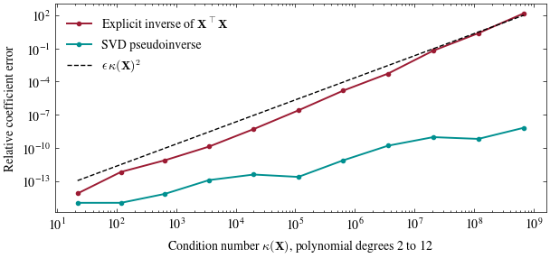
def polynomial_fit_errors(degree, n=60): t = np.linspace(0, 1, n) X = np.vander(t, degree +1, increasing=True) w_true = np.random.default_rng(degree).normal(0, 1, degree +1) y = X @ w_true w_inv = np.linalg.inv(X.T @ X) @ X.T @ y w_svd = np.linalg.pinv(X) @ y size = np.abs(w_true).max()return (np.linalg.cond(X), np.abs(w_inv - w_true).max() / size, np.abs(w_svd - w_true).max() / size)degrees = np.arange(2, 13)conds, err_inv, err_svd = np.array([polynomial_fit_errors(k) for k in degrees]).Tfig, ax = plt.subplots(figsize=(7, 3))ax.plot(conds, err_inv, color=CARDINAL, marker="o", markersize=3, linewidth=1.4, label="Explicit inverse of $\\mathbf{X}^\\top\\mathbf{X}$")ax.plot(conds, err_svd, color=TEAL, marker="o", markersize=3, linewidth=1.4, label="SVD pseudoinverse")ax.plot(conds, np.finfo(float).eps * conds **2, color="black", linestyle="--", linewidth=1.0, label="$\\epsilon \\, \\kappa(\\mathbf{X})^2$")ax.set_xscale("log")ax.set_yscale("log")ax.set_xlabel("Condition number $\\kappa(\\mathbf{X})$, polynomial degrees 2 to 12")ax.set_ylabel("Relative coefficient error")ax.legend(frameon=False)plt.show()
The explicit inverse tracks \(\epsilon\,\kappa(\mathbf{X})^2\) across seven orders of magnitude in \(\kappa(\mathbf{X})\), where \(\epsilon \approx 2\times10^{-16}\) is machine precision: it loses digits at the rate the squared condition number predicts. The pseudoinverse stays near machine precision the whole way. By degree \(12\) the two answers differ by ten orders of magnitude, running the same formula on the same data.
What if we push the degree further?
Change degree below and re-run. Degree \(9\) still looks respectable and degree \(12\) does not; push past \(14\) and the explicit inverse returns coefficients with no relationship to the ones we chose, while the SVD keeps degrading gracefully.
degree =12# change me!cond, rel_inv, rel_svd = polynomial_fit_errors(degree)print(f"degree {degree}")print(f" condition number of X: {cond:.3e}")print(f" condition number of X^T X: {cond **2:.3e}")print(f" relative error, inverse: {rel_inv:.3e}")print(f" relative error, SVD: {rel_svd:.3e}")
degree 12
  condition number of X:     6.771e+08
  condition number of X^T X: 4.585e+17
  relative error, inverse:   1.499e+02
  relative error, SVD:       6.578e-09
Punchline: all three solvers compute the same projection in theory, and the condition number of \(\mathbf{X}\) decides how much that theory is worth in practice. Forming \(\mathbf{X}^\top\mathbf{X}\) squares it, which costs the closed form its digits, and that same squared number stretches the bowl, which costs gradient descent its steps. The SVD and rescaled features are two ways of refusing to square the condition number.