Optimization

Last lecture fixed the model class, linear in the weights however we featurize the inputs, and left us staring at a picture. Predictions \(\hat{\mathbf{y}} = \mathbf{X}\mathbf{w}\) live in the column space of the design matrix \(\mathbf{X} \in \mathbb{R}^{n \times d}\), mean squared error measures the distance from the labels \(\mathbf{y} \in \mathbb{R}^n\) down to that subspace, and the best fit is the projection of \(\mathbf{y}\) onto it. We know exactly what we are looking for; we have not said how to compute it.

How do we actually find the weights that minimize mean squared error, and what does finding them cost?

There are two routes, a closed-form formula and gradient descent, and one number governs both: the condition number of the design matrix, \[ \kappa(\mathbf{X}) = \frac{\sigma_{\max}}{\sigma_{\min}}, \] the ratio of the largest to the smallest singular value of \(\mathbf{X}\), from the Decompositions lecture. It decides how many digits the exact formula keeps and how many steps the iteration takes.

Squared Error Is a Bowl

Write the loss in the design-matrix form we set up last lecture: \[ \mathcal{L}(\mathbf{w}) = \frac1n\|\mathbf{X}\mathbf{w} - \mathbf{y}\|_2^2 , \] where \(\mathbf{w} \in \mathbb{R}^d\) is the weight vector. Problem 3 already handed us its gradient: \[ \nabla_\mathbf{w} \mathcal{L}(\mathbf{w}) = \frac2n \mathbf{X}^\top(\mathbf{X}\mathbf{w} - \mathbf{y}). \] The vector \(\mathbf{X}\mathbf{w} - \mathbf{y} \in \mathbb{R}^n\) is the residual, one entry per data point, and multiplying by \(\mathbf{X}^\top\) measures how much each feature correlates with it: the gradient’s \(j\)th entry is large exactly when feature \(j\) still lines up with what the model is missing.

Problem 3 also showed that the matrix \(\mathbf{X}^\top\mathbf{X} \in \mathbb{R}^{d\times d}\) is positive semi-definite: for any direction \(\mathbf{v} \in \mathbb{R}^d\), \[ \mathbf{v}^\top(\mathbf{X}^\top\mathbf{X})\mathbf{v} = (\mathbf{X}\mathbf{v})^\top(\mathbf{X}\mathbf{v}) = \|\mathbf{X}\mathbf{v}\|_2^2 \geq 0 . \] Since \(\frac2n\mathbf{X}^\top\mathbf{X}\) is the matrix of second derivatives of \(\mathcal{L}\), the curvature of the loss is nonnegative in every direction: \(\mathcal{L}\) is convex, a bowl facing up, with no ridges and no saddles, so a point where the gradient vanishes is the global minimum.

The Normal Equations

So we set the gradient to zero at the minimizer \(\mathbf{w}^\star\) and solve, one move per line: \[ \begin{align*} \frac2n \mathbf{X}^\top(\mathbf{X}\mathbf{w}^\star - \mathbf{y}) &= \mathbf{0} \\ \mathbf{X}^\top(\mathbf{X}\mathbf{w}^\star - \mathbf{y}) &= \mathbf{0} \\ \mathbf{X}^\top\mathbf{X}\mathbf{w}^\star &= \mathbf{X}^\top\mathbf{y} \\ \mathbf{w}^\star &= (\mathbf{X}^\top\mathbf{X})^{-1}\mathbf{X}^\top\mathbf{y} . \end{align*} \] The first move multiplies both sides by \(n/2\); the second distributes \(\mathbf{X}^\top\); the third multiplies on the left by \((\mathbf{X}^\top\mathbf{X})^{-1}\), assuming for the moment that the inverse exists. The middle line has a name. The normal equations are the linear system \[ \mathbf{X}^\top\mathbf{X}\mathbf{w}^\star = \mathbf{X}^\top\mathbf{y} , \] \(d\) equations in the \(d\) unknowns of \(\mathbf{w}^\star\). This is the derivation we do at the board in class, and it lands on the answer last lecture’s picture implied: the line above the last, \(\mathbf{X}^\top(\mathbf{X}\mathbf{w}^\star - \mathbf{y}) = \mathbf{0}\), says every column of \(\mathbf{X}\) has inner product zero with the residual, which is exactly “drop a perpendicular from \(\mathbf{y}\) to the column space.” Problem 7 has you check that the two agree line for line.

When does the inverse we assumed actually exist? The chain above answers that too: \(\mathbf{v}^\top(\mathbf{X}^\top\mathbf{X})\mathbf{v} = \|\mathbf{X}\mathbf{v}\|_2^2\) is zero exactly when \(\mathbf{X}\mathbf{v} = \mathbf{0}\), so the inverse exists exactly when the \(d\) columns are linearly independent, which requires at least \(d\) data points; that is the case we work in today. When \(d > n\), the question we planted last lecture, infinitely many weight vectors fit the data exactly and the formula has nothing to say about which to pick; the Generalization lecture picks one and shows the choice matters more than it sounds. For now we have a formula and no sense of what it costs to evaluate.

The Cost of an Exact Answer

Written as one line of algebra the closed form looks free; let’s count the arithmetic, as we’ll do live in class, with \(n\) data points and \(d\) features.

Forming \(\mathbf{X}^\top\mathbf{X} \in \mathbb{R}^{d\times d}\) means filling in \(d^2\) entries, and entry \((j,k)\) is the inner product of columns \(j\) and \(k\) of \(\mathbf{X}\), two vectors of length \(n\), costing \(n\) multiplications and \(n-1\) additions. That is \(O(n)\) per entry and \(O(nd^2)\) in total. Forming \(\mathbf{X}^\top\mathbf{y} \in \mathbb{R}^d\) is \(d\) inner products of length \(n\), so \(O(nd)\). Solving the \(d\times d\) system by Gaussian elimination sweeps \(d\) columns, and each sweep updates a block of up to \(d^2\) entries, so \(O(d^3)\). Adding the three and dropping the term that is dominated by the others: \[ O(nd^2 + d^3) . \] Doubling \(n\) doubles the work, but doubling \(d\) multiplies it by eight: features, not data points, are what make this formula expensive, which is worth remembering the next time a feature map tempts us into a few thousand polynomial terms. At \(n = 10^6\) and \(d = 10^4\), the term \(nd^2\) alone is \(10^{14}\) operations, a fit that finishes overnight instead of during lecture. (In practice nobody computes \((\mathbf{X}^\top\mathbf{X})^{-1}\) and then multiplies; solving the system \(\mathbf{X}^\top\mathbf{X}\mathbf{w}^\star = \mathbf{X}^\top\mathbf{y}\) directly is the same \(O(d^3)\) with better constants and accuracy.)

Runtime is the cost an operation count can see. Forming \(\mathbf{X}^\top\mathbf{X}\) has a second cost that it cannot.

Two Ways to Solve: Inverse or SVD

Computers store real numbers with about \(16\) significant decimal digits, and every arithmetic operation rounds. Solving along the smallest singular direction divides by \(\sigma_{\min}\), amplifying whatever rounding error rode in on the data; the rule of thumb is that solving a system with condition number \(\kappa\) costs roughly \(\log_{10}\kappa\) significant digits. A design matrix with \(\kappa(\mathbf{X}) = 10^4\), unremarkable when one feature is in dollars and another in millions of dollars, costs four digits out of sixteen: affordable.

The trouble is that the normal equations do not solve a system with \(\mathbf{X}\) in it. They solve one with \(\mathbf{X}^\top\mathbf{X}\). Substitute the SVD \(\mathbf{X} = \sum_i \sigma_i \mathbf{u}_i \mathbf{v}_i^\top\) from the Decompositions lecture and use orthonormality of the left singular vectors, \(\mathbf{u}_i^\top\mathbf{u}_j = 1\) when \(i = j\) and \(0\) otherwise: \[ \mathbf{X}^\top\mathbf{X} = \Big(\sum_i \sigma_i \mathbf{v}_i\mathbf{u}_i^\top\Big)\Big(\sum_j \sigma_j \mathbf{u}_j\mathbf{v}_j^\top\Big) = \sum_{i,j} \sigma_i\sigma_j\, \mathbf{v}_i (\mathbf{u}_i^\top\mathbf{u}_j) \mathbf{v}_j^\top = \sum_i \sigma_i^2\, \mathbf{v}_i\mathbf{v}_i^\top . \] The double sum collapses because only the \(i = j\) terms survive. What is left is an eigendecomposition: the eigenvectors of \(\mathbf{X}^\top\mathbf{X}\) are the right singular vectors of \(\mathbf{X}\) and its eigenvalues are the squared singular values, exactly the link we verified by hand in the Decompositions lecture. Its condition number is therefore \[ \kappa(\mathbf{X}^\top\mathbf{X}) = \frac{\sigma_{\max}^2}{\sigma_{\min}^2} = \kappa(\mathbf{X})^2 . \] That squaring doubles the digits we lose: the comfortable \(\kappa(\mathbf{X}) = 10^4\) becomes \(10^8\), and eight digits out of sixteen is half our precision spent before the solve begins.

The fix is to never form \(\mathbf{X}^\top\mathbf{X}\) at all, and the SVD lets us avoid it. Define the pseudoinverse of \(\mathbf{X}\) from its SVD by inverting each singular value in place: \[ \mathbf{X}^+ = \sum_i \frac{1}{\sigma_i}\mathbf{v}_i\mathbf{u}_i^\top \in \mathbb{R}^{d \times n} . \]

Claim: When \(\mathbf{X}\) has linearly independent columns, the pseudoinverse reproduces the normal-equations formula exactly, so \(\mathbf{w}^\star = \mathbf{X}^+\mathbf{y}\) is the least-squares solution.

Proof of Claim

Inverting the sum of outer products we just computed inverts each eigenvalue and leaves the eigenvectors alone, so \((\mathbf{X}^\top\mathbf{X})^{-1} = \sum_i \sigma_i^{-2}\mathbf{v}_i\mathbf{v}_i^\top\). Multiply it by \(\mathbf{X}^\top = \sum_j \sigma_j\mathbf{v}_j\mathbf{u}_j^\top\) and collapse the double sum with orthonormality of the right singular vectors: \[ \begin{align*} (\mathbf{X}^\top\mathbf{X})^{-1}\mathbf{X}^\top &= \Big(\sum_i \frac{1}{\sigma_i^2}\mathbf{v}_i\mathbf{v}_i^\top\Big)\Big(\sum_j \sigma_j \mathbf{v}_j\mathbf{u}_j^\top\Big) \\&= \sum_{i,j} \frac{\sigma_j}{\sigma_i^2}\, \mathbf{v}_i (\mathbf{v}_i^\top\mathbf{v}_j) \mathbf{u}_j^\top \\&= \sum_i \frac{\sigma_i}{\sigma_i^2}\, \mathbf{v}_i\mathbf{u}_i^\top \\&= \sum_i \frac{1}{\sigma_i}\mathbf{v}_i\mathbf{u}_i^\top = \mathbf{X}^+ . \end{align*} \] The first equality substitutes both outer-product forms, the second regroups so the inner product \(\mathbf{v}_i^\top\mathbf{v}_j\) sits in the middle, and the third keeps only the \(i = j\) terms.

The two formulas agree in exact arithmetic but differ in what a computer touches on the way: the pseudoinverse route divides by \(\sigma_i\) once, so its arithmetic only ever sees \(\kappa(\mathbf{X})\), while the normal-equations route squares every singular value first. This is why numpy.linalg.lstsq and numpy.linalg.pinv are built on the SVD.

The class demo makes the gap visible with the polynomial feature map from last lecture, pushing \(\kappa(\mathbf{X})\) high enough that the explicit inverse and the pseudoinverse, run on the same data, stop agreeing.

Gradient Descent: An Iterative Alternative

Both routes so far cost \(O(nd^2)\), because both build a \(d\times d\) matrix out of the data before they solve anything. But we are standing on the inside of a bowl and we want the bottom; we do not have to solve for it if we are willing to walk toward it. The gradient points in the direction that increases \(\mathcal{L}\) fastest, by its defining property from the Linear Algebra lecture, so stepping the opposite way decreases the loss: \[ \mathbf{w}^{(t+1)} = \mathbf{w}^{(t)} - \alpha \nabla_\mathbf{w}\mathcal{L}(\mathbf{w}^{(t)}), \] where the superscript \((t)\) indexes iterations and \(\alpha > 0\) is a learning rate, the length of one step. This is gradient descent. For mean squared error we know the gradient exactly, so the update is \[ \mathbf{w}^{(t+1)} = \mathbf{w}^{(t)} - \frac{2\alpha}{n}\mathbf{X}^\top\big(\mathbf{X}\mathbf{w}^{(t)} - \mathbf{y}\big) . \] Each iteration predicts, measures the residual, and nudges the weights; when nothing is missing, the step is zero and the iteration stops moving.

Now count what one step costs. The product \(\mathbf{X}\mathbf{w}^{(t)}\) is \(n\) inner products of length \(d\), so \(O(nd)\); subtracting \(\mathbf{y}\) is \(O(n)\); multiplying the result by \(\mathbf{X}^\top\) is another \(O(nd)\). A step is \(O(nd)\) and \(T\) steps are \[ O(Tnd) , \] against \(O(nd^2 + d^3)\) for the closed form. Iterating wins whenever \(T \ll d\), and it never forms \(\mathbf{X}^\top\mathbf{X}\), so it never squares the condition number either. Because \(\mathcal{L}\) is convex, repeated updates reach the same \(\mathbf{w}^\star\) the closed form computes, provided \(\alpha\) is small enough that a step does not fly past the bottom. We take convergence on faith today; the Gradient Descent lecture proves it and reuses this exact update for logistic regression and neural networks, where no closed form exists.

If gradient descent is cheaper per step and avoids the squared condition number, why did we spend two sections on the closed form? Because \(T\) is hiding a great deal.

The Shape of the Bowl

\(T\) can be large because a single learning rate has to serve every direction at once, and a bowl need not be equally steep in every direction. To see the shape we are walking on, measure position by the error \(\mathbf{e} = \mathbf{w} - \mathbf{w}^\star \in \mathbb{R}^d\) and expand the loss around its minimum: \[ \begin{align*} \mathcal{L}(\mathbf{w}^\star + \mathbf{e}) &= \frac1n\big\|(\mathbf{X}\mathbf{w}^\star - \mathbf{y}) + \mathbf{X}\mathbf{e}\big\|_2^2 \\&= \frac1n\|\mathbf{X}\mathbf{w}^\star - \mathbf{y}\|_2^2 + \frac2n\mathbf{e}^\top\mathbf{X}^\top(\mathbf{X}\mathbf{w}^\star - \mathbf{y}) + \frac1n\|\mathbf{X}\mathbf{e}\|_2^2 \\&= \mathcal{L}(\mathbf{w}^\star) + \frac1n\mathbf{e}^\top\mathbf{X}^\top\mathbf{X}\mathbf{e} . \end{align*} \] The first equality substitutes \(\mathbf{w} = \mathbf{w}^\star + \mathbf{e}\) and splits the vector inside the norm, the second expands the square of a sum, and the third drops the middle term because \(\mathbf{X}^\top(\mathbf{X}\mathbf{w}^\star - \mathbf{y}) = \mathbf{0}\) is exactly the normal equations. Now substitute the outer-product form \(\mathbf{X}^\top\mathbf{X} = \sum_i \sigma_i^2\mathbf{v}_i\mathbf{v}_i^\top\) we derived above: \[ \mathcal{L}(\mathbf{w}^\star + \mathbf{e}) - \mathcal{L}(\mathbf{w}^\star) = \frac1n\sum_i \sigma_i^2\,(\mathbf{v}_i^\top\mathbf{e})^2 = \frac12\sum_i \lambda_i\,(\mathbf{v}_i^\top\mathbf{e})^2 . \] The second equality just names the curvature of the loss along the right singular vector \(\mathbf{v}_i\): \[ \lambda_i = \frac{2\sigma_i^2}{n} . \] The excess loss is a sum of independent one-dimensional parabolas: moving along \(\mathbf{v}_i\) changes only the \(i\)th term. The bowl is steep along the top singular direction (\(\lambda_{\max}\)) and shallow along the bottom one (\(\lambda_{\min}\)), and its aspect ratio is the number we have been tracking all lecture: \[ \frac{\lambda_{\max}}{\lambda_{\min}} = \frac{\sigma_{\max}^2}{\sigma_{\min}^2} = \kappa(\mathbf{X})^2 . \] The \(\kappa(\mathbf{X})^2\) that limited the precision of the closed form is the same \(\kappa(\mathbf{X})^2\) that stretches the bowl gradient descent has to walk down. The two halves of the lecture are about one number.

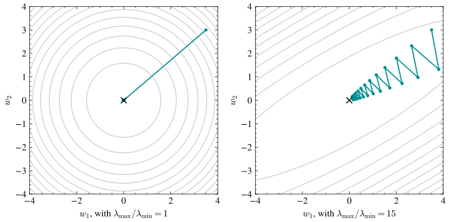
In the plot, both panels show the level sets of such a quadratic loss in two dimensions and the path gradient descent takes from the same starting point, with the minimum at the black cross. On the left the two curvatures are equal, the level sets are circles, and one step of the right size arrives. On the right the steep direction curves \(15\) times harder than the shallow one, the level sets stretch into a narrow valley, and the path zig-zags across it: a step size large enough to make progress down the shallow axis overshoots the steep axis and bounces off the opposite wall, so \(\alpha\) must be small enough for the steep direction, which leaves it far too small for the shallow one. The count of steps grows with the aspect ratio \(\lambda_{\max}/\lambda_{\min}\) and not with the number of parameters \(d\): a two-parameter problem with a stretched bowl is harder than a thousand-parameter problem with a round one. Problem 8 makes this precise and derives the exact rate, starting from a one-dimensional bowl and building up to this picture.

Fixing the Geometry Instead of the Step Size

The class demo watches this stretched bowl slow gradient descent on a two-feature dataset where one feature sits on a scale a thousand times larger than the other: the large-scale weight converges quickly and the small-scale one barely moves after tens of thousands of steps.

The repair is to change the bowl rather than the step size. Dividing each feature column by its standard deviation only rescales the columns, so the column space and the achievable minimum are unchanged, but it shrinks \(\kappa(\mathbf{X})\) toward \(1\) and rounds the bowl; the demo shows the rescaled run reaching the same minimum in a handful of steps. Rescaling costs one pass over the data and helps more here than any amount of tuning \(\alpha\), and it worked because our two features differed only in their units. What would you do if instead two features were near-duplicates of each other, so that \(\sigma_{\min}\) is small for a reason no choice of units can repair?

Looking Forward

The condition number limits the accuracy of the closed form and the speed of gradient descent, and it is not finished with us. The Gradient Descent lecture adds momentum, improving the dependence from \(\kappa\) to \(\sqrt{\kappa}\); the Depth-enablers lecture keeps a deep network’s Jacobians well conditioned; Muon builds an optimizer that flattens a matrix’s singular values to \(1\) before stepping; and the Generalization lecture traces the double-descent peak to a \(\sigma_{\min}\) near zero.

Both solvers minimize error on the data we already have. Next lecture questions whether that is the right thing to minimize: a model that fits the training data perfectly is not necessarily a good model, and we need an honest way to tell the difference.

Carry one sentence out of today: when a problem’s geometry is stretched, no single step size can serve every direction, so fix the geometry before you tune the step size.