Methodology
In the Regression lecture’s demo, a 13-parameter wiggle threaded perfectly through a month of ice-cream sales while a plain quadratic left visible gaps. On a fresh month generated by the same hidden function, the wiggle’s error exploded while the quadratic’s barely moved.
The only error we can compute is the error on data we have already used, and the only error we care about is the error on data we have not seen. Today we make the gap between those two numbers precise: where it comes from, how large it is, and how to measure the second one without fooling ourselves.
Generalization and the Three Splits
Generalization is a model’s performance on data it did not train on. It is what we actually care about (nobody deploys a model to re-predict the training set), yet fitting only ever gives us feedback on the data we fit to.
The standard fix is to hold data back. Split the dataset into three disjoint pieces: a training set used to fit the weights \(\mathbf{w}\), a validation set used to choose hyperparameters (like the polynomial degree), and a test set touched exactly once, at the very end, to report how the final model actually performs. To keep the three scores straight, recall the batch loss from the Mean Squared Error lecture, the mean squared error of a hypothesis \(f\) on a set \(S\) of labeled points: \[ \mathcal{L}_S(f) = \frac{1}{|S|}\sum_{i \in S} \big(y^{(i)} - f(\mathbf{x}^{(i)})\big)^2 . \] The three splits give three numbers for the one fitted model \(\hat f\): \(\mathcal{L}_{\text{train}}(\hat f)\), \(\mathcal{L}_{\text{val}}(\hat f)\), and \(\mathcal{L}_{\text{test}}(\hat f)\).
Why should an average over a few held-out days tell us anything about a customer we have never seen? Because it is the estimator from the Monte Carlo lecture, applied to squared error. Hold the fitted \(\hat f\) fixed: each validation point’s squared error \((y^{(i)} - \hat f(\mathbf{x}^{(i)}))^2\) is drawn from the same distribution as the error \(\hat f\) would suffer on any fresh point, so their average is a sample mean, unbiased for the quantity we actually want: \[ \mathbb{E}\big[\mathcal{L}_{\text{val}}(\hat f)\big] = \mathbb{E}\big[(y - \hat f(\mathbf{x}))^2\big], \] where the right side is the expected squared error on a single fresh point \((\mathbf{x}, y)\). By the \(1/\sqrt{n}\) rate from that same lecture, the score’s spread shrinks like \(1/\sqrt{n_{\text{val}}}\), so a small validation set gives an honest but noisy verdict. The argument used exactly one assumption, that \(\hat f\) never looked at these points, and the rest of this lecture is about protecting it.
Overfitting and Underfitting
Comparing training error to validation error diagnoses two opposite failure modes. Underfitting is high error on both training and validation data, because the model class is too weak to capture the pattern, the way a constant function underfits the ice-cream arc. Overfitting is low training error paired with high validation error, because the model has capacity to spare and spent it memorizing the training set’s particular noise rather than the pattern underneath.
As the polynomial degree grows, training error only ever decreases, a claim we prove below, while validation error bottoms out near the true degree and then climbs as higher-degree fits chase individual training points instead of the shared arc. The demo fits this family degree by degree on the ice-cream data and watches the two curves trace exactly that U-shape.
The training curve’s steady slide downward is not a quirk of this dataset. A larger menu can only offer a better best option.
Claim: Training error can only decrease (weakly) as the polynomial degree grows.
Proof of Claim
Let \(\mathcal{F}_k\) be the class of degree-\(k\) polynomials and \(\mathcal{F}_{k+1}\) the class of degree-\((k+1)\) polynomials, so \(\mathcal{F}_k \subset \mathcal{F}_{k+1}\): every degree-\(k\) polynomial is also a degree-\((k+1)\) polynomial, just with its degree-\((k+1)\) coefficient set to zero. Empirical risk minimization searches the entire model class for the minimizer, and \(\mathcal{F}_{k+1}\) contains everything \(\mathcal{F}_k\) contains and more, so the best achievable training error over the larger class can be no worse than over the smaller one: \[ \min_{f \in \mathcal{F}_{k+1}} \mathcal{L}_{\text{train}}(f) \;\leq\; \min_{f \in \mathcal{F}_k} \mathcal{L}_{\text{train}}(f) . \] Nesting the classes is what makes the inequality automatic, and nothing about polynomials was used: adding any feature to a linear model has the same effect, since the old weights are still available with a zero coefficient on the newcomer.Training error, by itself, cannot tell overfitting from a genuinely better fit, since it goes down (or stays flat) in both cases by the claim above. Only a validation set, held out from training, can tell the difference. That leaves the quantitative question the claim does not touch: by how much does training error mislead us?
The Optimism of Training Error
The mechanism is this: the fit slides toward the noise in the training labels, so the residuals it leaves behind are smaller than the noise really is. The smallest possible model class makes the size of that effect exact.
Take the class of constants \(f(x) = c\) from the Regression lecture, and suppose the truth is a constant too, so that the \(n\) training labels are: \[ y^{(i)} = \mu + \eta^{(i)}, \qquad \eta^{(i)} \sim \mathcal{N}(0, \sigma^2) \ \text{ independent}, \] where \(\mu \in \mathbb{R}\) is the unknown constant and \(\sigma^2\) is the noise level. The Mean Squared Error lecture showed the constant minimizing squared error is the sample mean, so \(\hat f(x) = \bar y = \mu + \bar\eta\), writing \(\bar\eta\) for the average of the \(n\) training noises. We can now compute what the training score says about this fit: \[ \begin{align*} \mathbb{E}\big[\mathcal{L}_{\text{train}}(\hat f)\big] &= \frac1n\sum_{i=1}^n \mathbb{E}\big[(y^{(i)} - \bar y)^2\big] \\&= \frac1n\sum_{i=1}^n \mathbb{E}\big[(\eta^{(i)} - \bar\eta)^2\big] \\&= \frac1n\sum_{i=1}^n \Big( \mathbb{E}\big[(\eta^{(i)})^2\big] - 2\,\mathbb{E}\big[\eta^{(i)}\bar\eta\big] + \mathbb{E}\big[\bar\eta^2\big] \Big) \\&= \sigma^2 - \frac{2\sigma^2}{n} + \frac{\sigma^2}{n} \;=\; \sigma^2\Big(1 - \frac1n\Big) . \end{align*} \] Here \(\mu\) cancels in the second equality, and the last uses \(\mathbb{E}[(\eta^{(i)})^2] = \sigma^2\), the sample-mean rate \(\mathbb{E}[\bar\eta^2] = \sigma^2/n\) from the Monte Carlo lecture, and \(\mathbb{E}[\eta^{(i)}\bar\eta] = \sigma^2/n\) by expanding \(\bar\eta\) and using independence.
Now score the very same \(\hat f\) on a fresh day, \(y = \mu + \eta\), whose noise \(\eta\) is independent of the whole training set: \[ \mathbb{E}\big[(y - \bar y)^2\big] = \mathbb{E}\big[(\eta - \bar\eta)^2\big] = \mathbb{E}[\eta^2] + \mathbb{E}\big[\bar\eta^2\big] = \sigma^2 + \frac{\sigma^2}{n} = \sigma^2\Big(1 + \frac1n\Big), \] where the cross term dropped this time because the fresh noise is independent of the training noises. Subtracting the two lines gives the gap between what we can measure and what we care about: \[ \sigma^2\Big(1 + \frac1n\Big) - \sigma^2\Big(1 - \frac1n\Big) = \frac{2\sigma^2}{n} . \] The optimism is systematic: averaged over training sets, the training score sits below the fresh-data score by a definite amount, wherever the truth \(\mu\) sits. The same computation for a linear model with \(d\) parameters gives an expected training error of \(\sigma^2(1 - d/n)\) and an optimism of \(2\sigma^2 d/n\): every parameter we fit absorbs a little more of the training noise, until at \(d = n\) the reported training error is exactly zero.
Problem 9 shows this is not special to constants: for any model class rich enough to contain the truth, the maximum likelihood estimate of \(\sigma^2\) built from training residuals comes out biased low. The optimism explains the training curve but not why the validation curve turns around and climbs; for that we need to name the two ways a fit can be wrong.
The Bias–Variance Decomposition
The U-curve has a name for each of its two halves, and the name comes from treating the training set itself as random. Imagine redrawing a fresh training set of the same size, refitting, and repeating many times; each refit produces a slightly different \(\hat f\), since each training set contains different noise. Averaged over these refits, the expected error at a fixed test point \(x\) splits into three pieces: \[ \mathbb{E}\big[(y - \hat f(x))^2\big] = \underbrace{\big(\mathbb{E}[\hat f(x)] - f^*(x)\big)^2}_{\text{bias}^2} + \underbrace{\mathrm{Var}(\hat f(x))}_{\text{variance}} + \underbrace{\mathrm{Var}(y \mid x)}_{\text{noise}} . \] Bias measures how far the average fitted function sits from the true \(f^*\), and is high for an underfit class too rigid to bend toward the truth no matter which training set it saw. Variance measures how much the fitted function itself swings from one training set to the next, and is high for an overfit class flexible enough to chase each training set’s particular noise. The last term is the spread of the label that survives after \(x\) is known; averaging it over test points as well recovers the irreducible error \(\mathbb{E}[\mathrm{Var}(Y \mid X)]\) from the Regression lecture.
Our constant-model computation is the whole decomposition in miniature. The bias is zero there, since the class contains the truth and the sample mean is unbiased; the variance is the familiar spread of a sample mean; and the noise is the noise: \[ \underbrace{0}_{\text{bias}^2} + \underbrace{\frac{\sigma^2}{n}}_{\text{variance}} + \underbrace{\sigma^2}_{\text{noise}} = \sigma^2\Big(1 + \frac1n\Big), \] which is exactly the fresh-day error we computed above. Bias and variance are properties of the model class and the amount of training data, not of the particular training set in front of us, which is why we cannot read either one off a single fit.
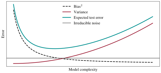
In the plot, bias\(^2\) falls as model complexity grows while variance climbs, and their sum traces the same U-shape, sitting on top of the noise floor it can never dip below. Problem 9 derives the decomposition in full, cross terms and all.
The bottom of the U sits at a complexity that depends on both \(f^*\) and \(\sigma^2\), neither of which we know, so it has to be found by searching.
Hyperparameter Search and Cross-Validation
The weights \(\mathbf{w}\) are parameters: the fitting procedure chooses them by empirical risk minimization on the training set. The polynomial degree is a hyperparameter, a knob the fitting procedure never touches, chosen from outside by comparing finished models. A regularization strength and last lecture’s learning rate \(\alpha\) are two more, and neural networks will bring a dozen others.
The search is the loop the demo runs. For each candidate value, fit on the training set, score that fit on the validation set, and keep the value with the smallest \(\mathcal{L}_{\text{val}}\). With two or three hyperparameters the same loop runs over a grid of combinations, at a cost of one full fit per grid point.
Holding out a validation set costs data, which hurts most when data is the scarce resource. Cross-validation stretches a small dataset further. Split the non-test data into \(k\) equal folds \(S_1, \ldots, S_k\); for each \(j\), fit a model \(\hat f^{(-j)}\) on every fold except the \(j\)th and score it on the fold it never saw: \[ \mathrm{CV}_k = \frac1k \sum_{j=1}^k \mathcal{L}_{S_j}\big(\hat f^{(-j)}\big) . \] Every point is used for validation exactly once and for training \(k-1\) times, and averaging \(k\) scores gives a steadier estimate than any single held-out fold. The cost is \(k\) full fits instead of one; \(k = 5\) or \(k = 10\) is the usual compromise, and \(k = n\) has its own name, leave-one-out. The \(k\) scores are not independent, since any two of their training sets overlap in all but two folds, so averaging them shrinks the independent part of their noise and leaves the shared part untouched. That is the correlation floor from Problem 1: averaging cannot remove the error that the folds share.
Whichever way we do it, the search looks at the validation data once per candidate, and that repetition has a cost.
Data Leakage and Honest Evaluation
If \(\mathcal{L}_{\text{val}}(\hat f)\) is an unbiased estimate of performance on fresh data, why do we need a third split at all? Because the number we would report is not the score of a model chosen in advance; it is the smallest of all the scores we looked at. Each candidate’s score is honest but wobbles around its own true error, and taking the minimum of many wobbling numbers systematically favors whichever candidate got lucky on the validation set. The optimism we quantified for training error returns one level up: fitting weights to the training set biases \(\mathcal{L}_{\text{train}}\) low, and selecting a hyperparameter on the validation set biases \(\mathcal{L}_{\text{val}}\) low. A test set exists so that the selection itself is graded by data that took no part in it, which makes \(\mathcal{L}_{\text{test}}(\hat f)\) the one number we can quote without an asterisk.
Data leakage is information from held-out data reaching the model, or reaching the decisions that produced the model. Peeking at the test set is the blatant version, and the subtle versions are the common ones. Standardizing features by the mean and standard deviation of the whole dataset before splitting leaks the held-out statistics into training; compute them on the training set alone and apply them to the other splits. Duplicate records that land on both sides of a split let a model score well by memorizing. Choosing which model class to try after seeing which one wins on the test data leaks the entire experiment. Tuning against “the test set” a dozen times and reporting the best run is \(p\)-hacking with a different name: a number that looks great and means nothing. The discipline of touching the test set exactly once, at the very end, is what keeps a reported accuracy connected to reality.
Looking Forward
Every model class in the rest of the course, logistic regression next lecture and neural networks after that, is judged by today’s standard: fit on one split, choose on a second, report on a third. Later in the semester, once models grow far past the number of training points, we will revisit the assumption baked into today’s U-curve, that capacity past the interpolation threshold can only make things worse, and find it is not quite true.
Carry one sentence out of today: any score computed on data that helped make a decision is optimistic about that decision, so the only honest number comes from data the decision never touched.