Demo: Gradient Descent on MNIST

Today’s labels are categorical rather than real: MNIST handwritten digits, \(0\) through \(9\). We build the softmax and cross-entropy machinery from the reading by hand, then fit it with plain gradient descent, which is the only option left once the closed form is gone.

import numpy as np
import matplotlib.pyplot as plt
import scienceplots
from matplotlib.colors import LinearSegmentedColormap
from sklearn.datasets import fetch_openml

plt.style.use(["science", "no-latex"])
TEAL, CARDINAL, GRAY = "#009090", "#9c1b33", "#c9c9c9"
CARDINAL_TEAL = LinearSegmentedColormap.from_list("cardinal_teal", [CARDINAL, "white", TEAL])
rng = np.random.default_rng(10)

X_all, y_all = fetch_openml("mnist_784", version=1, return_X_y=True, as_frame=False, parser="auto")
y_all = y_all.astype(int)

# subsample for a demo that trains in seconds, not minutes
idx = rng.choice(len(X_all), size=6000, replace=False)
X_all, y_all = X_all[idx], y_all[idx]
X_all = X_all / 255.0                      # pixels to [0, 1]
X_all = np.column_stack([X_all, np.ones(len(X_all))])   # fold in the bias column

n_train = 5000
X_train, y_train = X_all[:n_train], y_all[:n_train]
X_val, y_val = X_all[n_train:], y_all[n_train:]
print(f"training on {n_train} digits, validating on {len(X_val)}")

training on 5000 digits, validating on 1000

Build the one-hot labels, and implement the gradient exactly as derived in lecture: \(\nabla_{\mathbf{z}} \ell = \mathbf{p} - \mathbf{y}\), chained through \(\mathbf{z} = \mathbf{X}\mathbf{W}\) to give \(\frac{1}{n}\mathbf{X}^\top(\mathbf{P} - \mathbf{Y})\).

k = 10  # digit classes
d = X_train.shape[1]

def one_hot(y, k):
    Y = np.zeros((len(y), k))
    Y[np.arange(len(y)), y] = 1
    return Y

Y_train = one_hot(y_train, k)
Y_val = one_hot(y_val, k)

def softmax(Z):
    Z = Z - Z.max(axis=1, keepdims=True)   # for numerical stability; doesn't change the output
    expZ = np.exp(Z)
    return expZ / expZ.sum(axis=1, keepdims=True)

def cross_entropy(P, Y):
    return -np.mean(np.sum(Y * np.log(P + 1e-12), axis=1))

def accuracy(P, y):
    return np.mean(P.argmax(axis=1) == y)

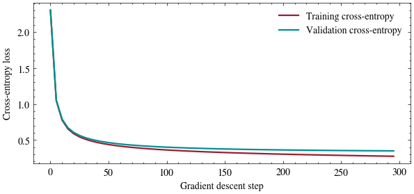
Now train. There is no closed form to fall back on, so we take \(300\) steps at \(\alpha = 0.5\) starting from \(\mathbf{W}^{(0)} = \mathbf{0}\), tracking both losses as we go.

W = np.zeros((d, k))
alpha = 0.5
n_steps = 300

steps, train_losses, val_losses, val_accs = [], [], [], []
for t in range(n_steps):
    P_train = softmax(X_train @ W)

    if t % 5 == 0:   # both scores measured at the same weights, before the step
        steps.append(t)
        train_losses.append(cross_entropy(P_train, Y_train))
        P_val = softmax(X_val @ W)
        val_losses.append(cross_entropy(P_val, Y_val))
        val_accs.append(accuracy(P_val, y_val))

    grad = X_train.T @ (P_train - Y_train) / n_train      # softmax minus one-hot, averaged
    W -= alpha * grad

fig, ax = plt.subplots(figsize=(7, 3))
ax.plot(steps, train_losses, color=CARDINAL, linewidth=1.6, label="Training cross-entropy")
ax.plot(steps, val_losses, color=TEAL, linewidth=1.6, label="Validation cross-entropy")
ax.set_xlabel("Gradient descent step")
ax.set_ylabel("Cross-entropy loss")
ax.legend(frameon=False)
plt.show()

print(f"final validation accuracy: {accuracy(softmax(X_val @ W), y_val):.1%}")

final validation accuracy: 90.9%

The validation curve pulls above the training curve and stays there: we are fitting \(785 \times 10 = 7{,}850\) parameters to \(5{,}000\) points, so the fit absorbs training noise the validation set never agreed to.

What did the model actually learn?

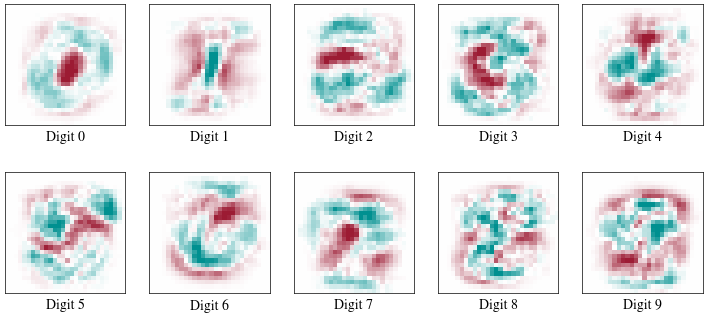
Each column of \(\mathbf{W}\) is a length-\(785\) weight vector for one digit class. Drop the bias entry, reshape the rest into a \(28 \times 28\) image, and look at it.

fig, axes = plt.subplots(2, 5, figsize=(9, 4))
for digit, ax in enumerate(axes.flat):
    weight_image = W[:-1, digit].reshape(28, 28)          # drop the bias row
    scale = np.percentile(np.abs(weight_image), 99)
    ax.imshow(weight_image, cmap=CARDINAL_TEAL, vmin=-scale, vmax=scale)
    ax.set_xlabel(f"Digit {digit}")
    ax.set_xticks([])
    ax.set_yticks([])
plt.show()

Teal pixels push that digit’s score up, cardinal pixels push it down. The column for \(0\) is a teal ring around a cardinal center, because ink in the middle of the frame is evidence against a zero; the column for \(1\) is a teal stripe down the middle with cardinal on either side. Each class gets exactly one template, which is all a linear model has room for.

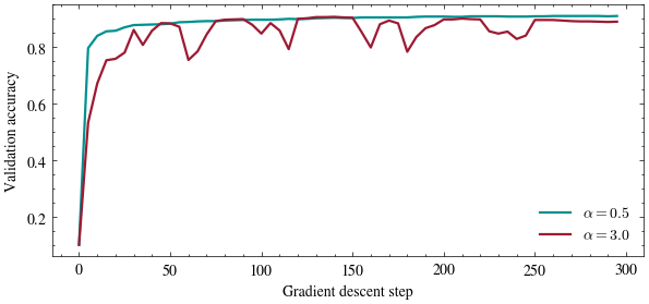
What if we used a bigger learning rate?

Change alpha_new below and re-run. Does a bigger step always get there sooner?

alpha_new = 3.0    # change me!

W2 = np.zeros((d, k))
val_accs2 = []
for t in range(n_steps):
    P_train = softmax(X_train @ W2)
    if t % 5 == 0:
        val_accs2.append(accuracy(softmax(X_val @ W2), y_val))
    W2 -= alpha_new * X_train.T @ (P_train - Y_train) / n_train

fig, ax = plt.subplots(figsize=(7, 3))
ax.plot(steps, val_accs, color=TEAL, linewidth=1.6, label=f"$\\alpha={alpha}$")
ax.plot(steps, val_accs2, color=CARDINAL, linewidth=1.6, label=f"$\\alpha={alpha_new}$")
ax.set_xlabel("Gradient descent step")
ax.set_ylabel("Validation accuracy")
ax.legend(frameon=False)
plt.show()

Punchline: a model with no hidden layers, no convolutions, and no closed-form solution reaches \(90.9\%\) on real handwritten digits using nothing but the softmax-minus-one-hot gradient we derived on paper. The accuracy left on the table is the linear decision boundary from the reading, and the Neural Networks unit spends its first lecture fixing it.