Logistic Regression
Every model this unit has built assumed the label \(y\) was a real number: cones sold, a house price. Today we close the unit with the other kind, the one the Regression lecture named and then set aside: spam or not spam, which digit is in the image. Regression asked “how much?”; classification asks “which one?”
The recipe from the Mean Squared Error lecture never actually mentioned regression: pick a model, commit to a distribution for the label, minimize the negative log-likelihood, and change nothing else when the distribution changes. Today we swap Gaussian for Bernoulli and follow the consequences: a new squashing function, a new loss, and one convenience lost along the way.
From a Score to a Probability
Start with binary labels, \(y \in \{0, 1\}\). The linear model from three lectures ago still applies, turning a feature vector into a single real number we will call the score: \[ z = \langle \mathbf{w}, \mathbf{x}\rangle \in \mathbb{R}, \] where \(\mathbf{x} \in \mathbb{R}^d\) is the feature vector and \(\mathbf{w} \in \mathbb{R}^d\) the weights, with the bias folded in as a constant feature as usual. A score is not a probability, so we need a function that squashes any real number into \((0,1)\), and the standard choice is the sigmoid function: \[ \sigma(z) = \frac{1}{1 + e^{-z}}. \]
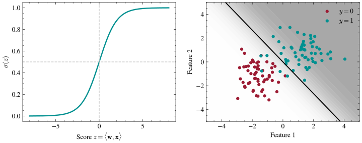
In the left panel, \(\sigma(z)\) slides smoothly from \(0\) to \(1\), crossing \(\frac12\) at \(z=0\): a score near zero is a shrug, and a large score is near-certainty that flattens. Our model now predicts: \[ f(\mathbf{x}) = \sigma\big(\langle \mathbf{w}, \mathbf{x}\rangle\big), \] read as the probability that \(y = 1\) given \(\mathbf{x}\). Why this particular squashing function, rather than any other S-shaped curve? Problem 10 derives it, starting from Bayes’ rule and assuming only that the features carry independent evidence, and arriving at exactly \(\sigma\) of a linear score.
Because \(\sigma(z) = \frac12\) exactly at \(z=0\), the predicted class flips wherever the score changes sign: the hyperplane \(\langle \mathbf{w}, \mathbf{x}\rangle = 0\) splits \(\mathbb{R}^d\) into a “predict \(1\)” half-space and a “predict \(0\)” half-space. The right panel shows this decision boundary for two features, with the background shading giving the predicted probability over two point clouds. The boundary where the shading crosses \(\frac12\) is a straight line, because the model underneath is still linear and only its output has been reinterpreted.
If the prediction only depends on the sign of the score, why bother with the sigmoid at all? A probability is more useful than a verdict: a doctor ordering a second test needs to know whether the model said \(0.51\) or \(0.99\). And a hard threshold has zero derivative almost everywhere, handing an optimizer no direction to move in, while the sigmoid is smooth enough to fit. To fit it, we need a loss.
The Likelihood of a Label
With a probability in hand, maximum likelihood works exactly as it did for regression, with one change: the noise model. A binary label is naturally modeled as a Bernoulli random variable with success probability \(f(\mathbf{x})\), and both of its cases fit in one expression: \[ \Pr(y \mid \mathbf{x}) = f(\mathbf{x})^{\,y}\,\big(1-f(\mathbf{x})\big)^{1-y}. \] Plug in \(y=1\) and the second factor becomes \(1\), and vice versa: the exponents are switches rather than arithmetic.
Now run the recipe from the Mean Squared Error lecture without changing a single step. The \(n\) labels are independent, so the likelihood of the dataset is a product, and a logarithm turns that product into a sum: \[ \begin{align*} \arg\max_\mathbf{w} \prod_{i=1}^n \Pr\big(y^{(i)} \mid \mathbf{x}^{(i)}\big) &= \arg\max_\mathbf{w} \sum_{i=1}^n \log \Pr\big(y^{(i)} \mid \mathbf{x}^{(i)}\big) \\&= \arg\max_\mathbf{w} \sum_{i=1}^n \Big[ y^{(i)} \log f(\mathbf{x}^{(i)}) + \big(1-y^{(i)}\big) \log\big(1 - f(\mathbf{x}^{(i)})\big) \Big]. \end{align*} \] The first equality is the Mean Squared Error lecture’s log moves, unchanged; the second substitutes the Bernoulli probability above and splits the logarithm, \(\log(a^y b^{1-y}) = y\log a + (1-y)\log b\). Flipping the sign turns the maximization into a minimization, and dividing by \(n\) moves nothing, so we are minimizing the binary cross-entropy loss: \[ \mathcal{L}(\mathbf{w}) = -\frac1n\sum_{i=1}^n \Big[ y^{(i)} \log f(\mathbf{x}^{(i)}) + \big(1-y^{(i)}\big) \log\big(1 - f(\mathbf{x}^{(i)})\big) \Big]. \] Each point pays \(-\log\) of the probability the model assigned to the correct answer, and nothing else: near zero when confident and right, unbounded as that probability approaches zero, so a single confident mistake can cost more than a hundred hedged ones. Gaussian noise handed us squared error and Bernoulli noise hands us cross-entropy, the same theorem run with a different distribution.
Binary labels were the easy case, and most classification problems have more than two answers: ten digits, or thousands of words.
Many Classes: Softmax and Categorical Cross-Entropy
Generalize the single score to a vector of \(k\) scores, one per class, called the logits: \[ \mathbf{z} = \mathbf{W}^\top\mathbf{x} \in \mathbb{R}^k, \] where the weight matrix \(\mathbf{W} \in \mathbb{R}^{d\times k}\) holds one column of weights per class, so that \(z_j = \langle [\mathbf{W}]_{,j}, \mathbf{x}\rangle\) is class \(j\)’s score. The softmax function turns these \(k\) scores into a probability distribution over the \(k\) classes: \[ [\mathrm{softmax}(\mathbf{z})]_j = \frac{e^{z_j}}{\sum_{l=1}^k e^{z_l}}, \] exponentiating so every entry is positive, then normalizing to sum to \(1\). Softmax sees only differences between logits (adding the same constant to every \(z_j\) cancels), and when one logit pulls far ahead its entry approaches \(1\), which is where the name comes from. Setting \(k=2\) and reading off the probability of class \(1\) recovers the sigmoid exactly. (Can you check that? Divide the numerator and denominator by \(e^{z_1}\) and compare with \(\sigma(z_1 - z_2)\).)
The label is now categorical, encoded as a one-hot vector: \[ \mathbf{y} \in \{0,1\}^k, \qquad \textstyle\sum_{j=1}^k y_j = 1, \] carrying its single \(1\) in the true class’s slot. The same likelihood recipe, with a categorical distribution in place of the Bernoulli, gives the categorical cross-entropy loss: \[ \mathcal{L}(\mathbf{W}) = -\frac1n\sum_{i=1}^n \sum_{j=1}^k y_j^{(i)} \log p_j^{(i)}, \qquad \mathbf{p}^{(i)} = \mathrm{softmax}\big(\mathbf{W}^\top\mathbf{x}^{(i)}\big), \] where \(\mathbf{p}^{(i)} \in \mathbb{R}^k\) is the model’s predicted distribution over classes for the \(i\)th point. Since \(\mathbf{y}^{(i)}\) is one-hot, only the true class’s log-probability survives the inner sum, so each point again pays \(-\log\) of the probability on the correct answer; the binary case is this formula at \(k=2\).
We have a model and a loss. Minimizing the loss needs its gradient.
The Cross-Entropy Gradient
The gradient comes out clean for a mechanical reason: cross-entropy takes a logarithm of something softmax built by exponentiating, so on the true class the two operations cancel and all that survives is the normalizer. We derive it at the board in class.
Claim: For a single example with logits \(\mathbf{z} \in \mathbb{R}^k\), one-hot label \(\mathbf{y}\) carrying its \(1\) in slot \(c\), and prediction \(\mathbf{p} = \mathrm{softmax}(\mathbf{z})\), the per-example cross-entropy \(\ell = -\log p_c\) has gradient \[ \nabla_\mathbf{z}\, \ell = \mathbf{p} - \mathbf{y}, \] which we read aloud as “softmax minus one-hot.”
Proof of Claim
Write \(\ell = -\log p_c = -z_c + \log \sum_{l=1}^k e^{z_l}\), using the definition of \(p_c\) and the logarithm of a quotient. Differentiate with respect to each logit \(z_j\). For the first term, \(\partial(-z_c)/\partial z_j\) is \(-1\) if \(j=c\) and \(0\) otherwise, which is exactly \(-y_j\). For the second term, the chain rule through the logarithm gives: \[ \frac{\partial}{\partial z_j} \log \sum_{l=1}^k e^{z_l} = \frac{e^{z_j}}{\sum_{l=1}^k e^{z_l}} = p_j. \] Adding the two pieces, \(\partial \ell/\partial z_j = p_j - y_j\) for every \(j\), which stacked into a vector is \(\nabla_\mathbf{z}\ell = \mathbf{p}-\mathbf{y}\).The gradient is the predicted distribution minus the true one, which is the residual of the Regression lecture written in probabilities instead of cones. It is zero exactly when the model already puts all of its mass on the true class, its most negative entry is always the true class’s own, \(p_c - 1\), and every entry lies in \([-1,1]\), so no single example can hand the logits an enormous gradient even though its loss is unbounded.
The gradient we can actually descend is the one on the weights, and the chain rule through \(\mathbf{z} = \mathbf{W}^\top\mathbf{x}\) delivers it. Logit \(z_j\) depends only on column \(j\) of \(\mathbf{W}\), and linearly, so \(\partial z_j / \partial [\mathbf{W}]_{,j} = \mathbf{x}\) and the per-example gradient is an outer product: \[ \nabla_\mathbf{W}\, \ell = \mathbf{x}\,(\mathbf{p} - \mathbf{y})^\top \in \mathbb{R}^{d \times k} . \] Averaging over the dataset gives the gradient of the loss itself: \[ \nabla_\mathbf{W}\mathcal{L}(\mathbf{W}) = \frac1n \sum_{i=1}^n \mathbf{x}^{(i)}\big(\mathbf{p}^{(i)} - \mathbf{y}^{(i)}\big)^\top = \frac1n \mathbf{X}^\top\big(\mathbf{P} - \mathbf{Y}\big), \] where \(\mathbf{X} \in \mathbb{R}^{n\times d}\) is the design matrix from the Linear Model lecture and \(\mathbf{P}, \mathbf{Y} \in \mathbb{R}^{n \times k}\) stack the predicted and one-hot distributions as rows; the second equality is the outer-product form of matrix multiplication from Unit 1.
That shape should surprise you: the least-squares gradient from the Optimization lecture was \(\frac{2}{n}\mathbf{X}^\top(\mathbf{X}\mathbf{w} - \mathbf{y})\), the design matrix transposed times a residual, again. The coincidence has one cause: in both cases the derivative of the loss with respect to the score is the residual, and the score is linear in the weights, so the chain rule multiplies that residual by \(\mathbf{x}\) and stops. The shape outlives this lecture: it is what backpropagation delivers at the output layer of every classifier we train in the next unit, and it is what the policy update looks like in the final unit, where “softmax minus one-hot” comes back scaled by a reward.
The gradient tells us how to push \(\mathbf{p}\) toward \(\mathbf{y}\), but not what quantity that push is shrinking, and cross-entropy’s name points straight at the answer.
Entropy and KL Divergence
Cross-entropy borrows its name from information theory, where the entropy of a distribution over \(k\) outcomes is the average surprise of a draw from it: \[ H(\mathbf{y}) = -\sum_{j=1}^k y_j \log y_j, \] where an outcome of probability \(y_j\) carries surprise \(-\log y_j\), so probability spread thinly over many outcomes means high entropy: a fair die has more entropy than a loaded one. The Kullback-Leibler divergence measures the extra surprise we suffer by holding the distribution \(\mathbf{p}\) while outcomes actually arrive from \(\mathbf{y}\): \[ D_{\mathrm{KL}}(\mathbf{y} \,\|\, \mathbf{p}) = \sum_{j=1}^k y_j \log \frac{y_j}{p_j}. \] The cross-entropy of the pair is the total surprise we suffer under \(\mathbf{p}\) when reality is \(\mathbf{y}\): \[ \mathrm{CE}(\mathbf{y}, \mathbf{p}) = -\sum_{j=1}^k y_j \log p_j, \] which is exactly the per-example loss from two sections ago.
The identity relating the three is one line of algebra we do live in class.
Claim: For any two distributions \(\mathbf{y}\) and \(\mathbf{p}\) over the same \(k\) outcomes, cross-entropy splits into entropy plus divergence: \[ \mathrm{CE}(\mathbf{y}, \mathbf{p}) = H(\mathbf{y}) + D_{\mathrm{KL}}(\mathbf{y}\,\|\,\mathbf{p}). \]
Proof of Claim
Split the logarithm inside the divergence, \(\log(y_j/p_j) = \log y_j - \log p_j\), and separate the sum: \[ \begin{align*} D_{\mathrm{KL}}(\mathbf{y}\,\|\,\mathbf{p}) &= \sum_{j=1}^k y_j \log y_j - \sum_{j=1}^k y_j \log p_j \\&= -H(\mathbf{y}) + \mathrm{CE}(\mathbf{y}, \mathbf{p}), \end{align*} \] where the second equality reads the definitions of \(H\) and \(\mathrm{CE}\) backwards, and rearranging gives the claim.Cross-entropy counts the surprise nobody could have avoided, the entropy, plus the extra surprise we brought on ourselves by predicting \(\mathbf{p}\) instead of \(\mathbf{y}\), and only the second piece contains the model. When we train, \(\mathbf{y}^{(i)}\) is a one-hot label, its entropy is \(0\) because no surprise is left once the answer is certain (with \(0\log 0 = 0\)), and the entire loss is a divergence: \[ \mathcal{L}(\mathbf{W}) = \frac1n\sum_{i=1}^n D_{\mathrm{KL}}\big(\mathbf{y}^{(i)} \,\|\, \mathbf{p}^{(i)}\big). \] So minimizing cross-entropy is distribution matching, pulling each \(\mathbf{p}^{(i)}\) onto the truth \(\mathbf{y}^{(i)}\) as measured by KL divergence, which is why KL appears whenever one distribution has to imitate another; we will use it again in the final unit, where a KL leash keeps a policy update from wandering too far from the action distribution it started with.
KL says what we are minimizing. It does not say how, and here the recipe finally costs us something.
Fitting by Gradient Descent
Every model in this unit so far could be fit in closed form, and this one cannot. Setting the gradient to zero gives \(\mathbf{X}^\top\mathbf{P} = \mathbf{X}^\top\mathbf{Y}\), but every entry of \(\mathbf{P}\) depends on \(\mathbf{W}\) through the softmax’s exponentials, and no rearrangement isolates \(\mathbf{W}\) the way the normal equations isolated \(\mathbf{w}^\star\). Gradient descent, introduced two lectures ago as one option out of two, is now the only option: \[ \mathbf{W}^{(t+1)} = \mathbf{W}^{(t)} - \frac{\alpha}{n}\,\mathbf{X}^\top\big(\mathbf{P}^{(t)} - \mathbf{Y}\big), \] where \(\alpha > 0\) is the learning rate from that lecture and \(\mathbf{P}^{(t)} \in \mathbb{R}^{n\times k}\) holds the predicted distributions at the current weights \(\mathbf{W}^{(t)}\).
Losing the closed form costs less than it sounds, because cross-entropy is convex in \(\mathbf{W}\), the same property that made least squares a bowl, so gradient descent still walks to a global minimum. One step is also cheap: \(O(ndk)\), dominated by forming \(\mathbf{X}\mathbf{W}\) and \(\mathbf{X}^\top(\mathbf{P}-\mathbf{Y})\), so \(T\) steps cost \(O(Tndk)\) against the \(O(nd^2 + d^3)\) the closed form would have cost.
The class demo runs exactly this update on MNIST digit images, tracking training against validation loss and then looking at what the fitted weights turn out to encode.
Looking Forward
The decision boundary in the last figure is always a hyperplane, for the same reason the weight matrix \(\mathbf{W}\) has only \(k\) columns: each class gets one linear score, computed against the whole input at once, so the best it can do is one template per class, scored by match. That limit is why no linear model can separate data that is not linearly separable, like the XOR pattern on four points, which you will prove is out of reach next lecture. The Neural Networks unit begins there, stacking simple nonlinear pieces until the boundary can bend, and it keeps today’s softmax-and-cross-entropy output layer on top of essentially every classifier for the rest of the course.
Carry one sentence out of today: the kind of label picks the distribution, the distribution picks the loss, and the rest of the machinery is the same.