Neural Networks
The Linear Models unit ended on a limitation: however we squash a linear score, the decision boundary underneath stays a flat hyperplane. Welcome to the Neural Networks unit, where we let go of that constraint. Until now we chose features first, then fit a linear model on top; a neural network learns the features and the final combination simultaneously. The unit takes four lectures: what a network is and how to differentiate it (today), then how to optimize it, what breaks when it gets deep, and why it generalizes.
The expressive half costs one new idea, a nonlinear function placed between two linear maps; the trainable half costs nothing new, because the chain rule from the Linear Algebra lecture already does the work.
Why Linear Models Are Not Enough
The smallest dataset that defeats a linear model has four points. XOR labels the corners of the unit square by whether exactly one of the two coordinates is \(1\): \[ (0,0) \mapsto 0, \qquad (1,0) \mapsto 1, \qquad (0,1) \mapsto 1, \qquad (1,1) \mapsto 0. \]
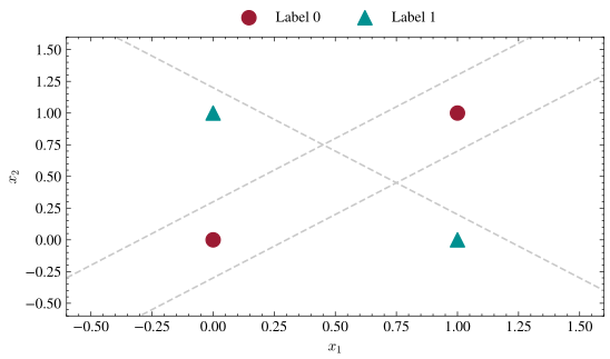
Claim: No linear decision boundary separates the XOR labels.
Proof of Claim
Suppose some line \(w_1 x_1 + w_2 x_2 + b = 0\) correctly separated the two classes, positive on the label-\(1\) side. Then \(w_1\cdot 1 + w_2 \cdot 0 + b > 0\) and \(w_1 \cdot 0 + w_2 \cdot 1 + b > 0\) (both label-\(1\) points), while \(w_1\cdot 0+w_2\cdot 0+b < 0\) and \(w_1\cdot 1+w_2\cdot 1+b<0\) (both label-\(0\) points). Adding the two label-\(1\) inequalities gives \(w_1+w_2+2b > 0\). Adding the two label-\(0\) inequalities gives \(w_1+w_2+2b < 0\). These two conclusions contradict each other, so no such line exists.Proving it is today’s first exercise at the board, the proof last lecture promised; check the block above afterward. In the plot, each dashed line we might try leaves a teal label-\(1\) point on the same side as a cardinal label-\(0\) point. The fix is to give the model several cuts, plus something nonlinear to combine them with. Last lecture’s closing example, two interleaved spirals, fails the same way; we come back to those once we have a model that can handle them.
A Neuron: Linear Map Plus Nonlinearity
A neuron is a linear map followed by a nonlinearity. On an input \(\mathbf{x} \in \mathbb{R}^d\) it computes the single number \[ a\big(\langle\mathbf{w},\mathbf{x}\rangle + b\big), \] where \(\mathbf{w}\in\mathbb{R}^d\) is a weight vector, \(b\in\mathbb{R}\) is a bias, and \(a:\mathbb{R}\to\mathbb{R}\) is the activation function, fixed in advance rather than learned. Three common choices:
- ReLU: \(a(z) = \max(0, z)\), zero for negative inputs and the identity for positive ones.
- Sigmoid: \(a(z) = \sigma(z) = \frac{1}{1+e^{-z}}\), the squashing function from last lecture.
- Tanh: \(a(z) = \tanh(z)\), shaped like the sigmoid but centered at \(0\) and ranging over \((-1,1)\).
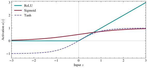
In the plot, all three curves are flat on the left and rising on the right. The sigmoid and tanh flatten out, so their derivatives fall to nearly zero once \(|z|\) is large, while ReLU keeps rising with slope \(1\) and bends only at \(z=0\). That single bend is the whole of ReLU’s nonlinearity, and it is the object Problem 11 spends its time counting.
(The step function \(a(z) = \mathbb{1}[z \geq 0]\) would encode “which side of the line” most cleanly, but its gradient is zero everywhere it is defined, so gradient descent has nothing to follow; ReLU keeps the flavor while staying differentiable almost everywhere.)
One neuron is still one cut with a bend at the end, no more expressive than logistic regression; everything beyond a hyperplane has to come from combining neurons.
Stacking Neurons into a Network
So we stack them. A layer applies many neurons to the same input at once, a matrix multiplication followed by an elementwise activation, and a multi-layer perceptron (MLP) feeds each layer’s outputs into the next as inputs. Writing \(\mathbf{h}^{(0)} = \mathbf{x}\) for the input and indexing layers with a parenthesized superscript, the network of \(L\) layers is defined by \[ \mathbf{h}^{(l)} = a\big(\mathbf{W}^{(l)}\mathbf{h}^{(l-1)} + \mathbf{b}^{(l)}\big), \qquad l = 1, \ldots, L, \] where layer \(l\) has \(d_l\) neurons, weight matrix \(\mathbf{W}^{(l)} \in \mathbb{R}^{d_l \times d_{l-1}}\), bias \(\mathbf{b}^{(l)} \in \mathbb{R}^{d_l}\), and an activation applied to each entry separately. The input layer has \(d_0 = d\) features; the last layer usually skips the activation so its output can be a real number (regression) or logits (classification, handed to last lecture’s softmax); every weight and bias is a parameter we train.
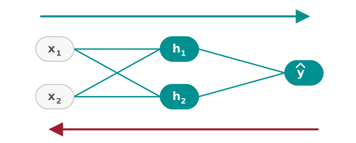
In the diagram, the gray pills are the input’s coordinates, the teal pills are neurons, and the teal edges the entries of the two weight matrices; the teal arrow is the forward pass turning \(\mathbf{x}\) into \(\hat y\), the cardinal arrow the backward pass we build in a moment, running the same edges in reverse.
Here is a network of exactly that shape, small enough to solve XOR by hand: \[ h_1 = \mathrm{ReLU}(x_1+x_2), \qquad h_2 = \mathrm{ReLU}(x_1+x_2-1), \qquad \hat y = h_1 - 2h_2 . \] Check all four corners:
| \((x_1,x_2)\) | \(h_1\) | \(h_2\) | \(\hat y = h_1-2h_2\) | XOR label |
| \((0,0)\) | \(0\) | \(0\) | \(0\) | \(0\) |
| \((1,0)\) | \(1\) | \(0\) | \(1\) | \(1\) |
| \((0,1)\) | \(1\) | \(0\) | \(1\) | \(1\) |
| \((1,1)\) | \(2\) | \(1\) | \(0\) | \(0\) |
Can you find a different pair of hidden neurons that also solves it?
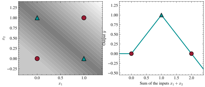
In the left panel, the shading is the network’s output over the whole square, with teal triangles at the label-\(1\) corners and cardinal circles at the label-\(0\) corners. Each hidden neuron contributes one crease, and the two creases together fold the flat output into a ridge running along the anti-diagonal. Both hidden neurons see the input only through the sum \(x_1+x_2\), so the output does too, and the right panel plots it against that sum: a tent that climbs from \(0\), peaks at height \(1\) when \(x_1+x_2=1\), and falls back through \(0\) at \(x_1+x_2=2\). The four corners land at heights \(0,1,1,0\), which is XOR.
This is the universal approximation intuition in miniature: enough creases can approximate essentially any function, and the classical theorem makes it precise, one hidden layer of sufficient width approximating any continuous function on a bounded domain to any accuracy. The theorem does not say how many neurons that takes, or whether gradient descent will find them; if one layer can approximate anything, why stack more? Problem 11 makes the “how many pieces” half of the question exact: a single hidden layer of width \(m\) folds a one-dimensional input into at most \(m+1\) flat pieces, while \(L\) layers of constant width reach \(2^L\) pieces by feeding the tent above into a copy of itself. Width adds pieces and depth multiplies them, so “enough neurons” in one layer can mean exponentially many.
Expressiveness, then, is not the obstacle; the other half of today’s question is whether we can still compute a gradient when the parameters sit several compositions deep.
The Chain Rule, Reviewed
Training a network still means gradient descent on a loss \(\mathcal{L}\), now a deep composition of functions rather than one linear map. Recall the chain rule for a scalar composition \(f(g(x))\): \[ \frac{\partial f}{\partial x} = \frac{\partial f}{\partial g}\cdot\frac{\partial g}{\partial x}. \] When \(f\) depends on \(x\) through \(m\) intermediate values \(g_1(x), \ldots, g_m(x)\), the multivariate chain rule collects one term per route from the input to the output: \[ \frac{\partial f}{\partial x} = \sum_{i=1}^m \frac{\partial f}{\partial g_i}\cdot\frac{\partial g_i}{\partial x}. \] A nudge to \(x\) reaches \(f\) along \(m\) separate paths, each multiplying the nudge by the sensitivities of its own links, and the total effect is the sum over all of them. The Linear Algebra lecture promised this moment: the chain rule returns with a matrix in place of each scalar factor.
Backpropagation applies the rule systematically: compute and store every intermediate value on a forward pass, then walk backward through the network, computing each layer’s gradients from those already computed one layer downstream.
Backpropagation by Hand
Let’s run both passes on one input, exactly as we will at the board. Take a \(2\)-input, \(2\)-hidden-neuron, \(1\)-output network with weights \[ \mathbf{W}^{(1)} = \begin{bmatrix} 1 & -1 \\ 1 & 1 \end{bmatrix}, \quad \mathbf{b}^{(1)} = \begin{bmatrix}0\\0\end{bmatrix}, \quad \mathbf{w}^{(2)} = \begin{bmatrix}1 \\ -1\end{bmatrix}, \quad b^{(2)} = 0, \] writing the single output neuron’s weights as a vector \(\mathbf{w}^{(2)}\in\mathbb{R}^2\) rather than a \(1\times 2\) matrix. Take input \(\mathbf{x} = (1,2)\), target \(y=1\), and squared error as the loss: \[ \mathcal{L} = (\hat y - y)^2 . \]
Forward pass. Push the input through the first layer and then the ReLU, writing \(\mathbf{z}^{(1)}\) for the pre-activations and \(\mathbf{h}\) for the hidden activations: \[ \mathbf{z}^{(1)} = \mathbf{W}^{(1)}\mathbf{x} + \mathbf{b}^{(1)} = \begin{bmatrix}1\cdot1 + (-1)\cdot 2 \\ 1\cdot 1 + 1\cdot 2\end{bmatrix} = \begin{bmatrix}-1\\3\end{bmatrix}, \qquad \mathbf{h} = \mathrm{ReLU}(\mathbf{z}^{(1)}) = \begin{bmatrix}0\\3\end{bmatrix}. \] Combine the two hidden activations with the output weights, and the loss follows: \[ \hat y = \langle \mathbf{w}^{(2)}, \mathbf{h}\rangle + b^{(2)} = 1\cdot 0 + (-1)\cdot 3 = -3, \qquad \mathcal{L} = (-3-1)^2 = 16. \]
Backward pass. Start at the output, where the derivative of the loss is immediate: \[ \frac{\partial \mathcal{L}}{\partial \hat y} = 2(\hat y - y) = 2(-3-1) = -8 . \] Push that number through the output layer, once for the weights it multiplied and once for the activations it multiplied: \[ \nabla_{\mathbf{w}^{(2)}} \mathcal{L} = \frac{\partial \mathcal{L}}{\partial \hat y}\cdot \mathbf{h} = -8 \begin{bmatrix}0\\3\end{bmatrix} = \begin{bmatrix}0\\-24\end{bmatrix}, \qquad \nabla_{\mathbf{h}} \mathcal{L} = \frac{\partial \mathcal{L}}{\partial \hat y}\cdot \mathbf{w}^{(2)} = -8\begin{bmatrix}1\\-1\end{bmatrix} = \begin{bmatrix}-8\\8\end{bmatrix}. \] The weight gradient updates each output weight in proportion to the hidden activation it multiplied, and the activation gradient sends the same error backward along the weights that carried it forward.
Next, push through the ReLU, whose derivative is \(1\) where \(z^{(1)}_i > 0\) and \(0\) where \(z^{(1)}_i < 0\), so the gradient is masked entry by entry: \[ \nabla_{\mathbf{z}^{(1)}}\mathcal{L} = \nabla_{\mathbf{h}}\mathcal{L} \odot \begin{bmatrix}\mathbb{1}[z_1^{(1)}>0]\\\mathbb{1}[z_2^{(1)}>0]\end{bmatrix} = \begin{bmatrix}-8\\8\end{bmatrix}\odot\begin{bmatrix}0\\1\end{bmatrix} = \begin{bmatrix}0\\8\end{bmatrix}, \] where \(\odot\) is entrywise multiplication. The first hidden neuron was inactive (\(z_1^{(1)}=-1<0\)), so its gradient is killed entirely, and every weight feeding it will sit unchanged through this step. That is a preview of a problem the Depth-enablers lecture spends a whole session on.
Finally, push through the first layer: \[ \nabla_{\mathbf{W}^{(1)}}\mathcal{L} = (\nabla_{\mathbf{z}^{(1)}}\mathcal{L})\,\mathbf{x}^\top = \begin{bmatrix}0\\8\end{bmatrix}\begin{bmatrix}1 & 2\end{bmatrix} = \begin{bmatrix}0&0\\8&16\end{bmatrix}, \qquad \nabla_{\mathbf{b}^{(1)}}\mathcal{L} = \nabla_{\mathbf{z}^{(1)}}\mathcal{L} = \begin{bmatrix}0\\8\end{bmatrix}. \] That last weight gradient is an outer product, the object the Linear Algebra lecture built out of one column and one row: entry \((i,j)\) is neuron \(i\)’s incoming error times input \(j\). These four arrays are everything one gradient descent step needs: subtract \(\alpha\) times each from the corresponding parameter.
We used squared error to keep the arithmetic small; for classification only the first line changes. The last layer produces a vector of logits \(\mathbf{z}\), and last lecture’s derivation hands us the starting gradient: \[ \nabla_{\mathbf{z}}\mathcal{L} = \mathbf{p} - \mathbf{y} , \] where \(\mathbf{p} = \mathrm{softmax}(\mathbf{z})\) is the predicted distribution over classes and \(\mathbf{y}\) is the one-hot label. Softmax minus one-hot replaces the single number above, and every line below it is identical, which is exactly where the demo starts.
The Matrix View
Every step of both passes was one small matrix operation, none of it tied to layers of exactly two neurons, and writing the pattern in matrix form is what makes networks fast. Take any two adjacent layers: write \(\mathbf{u}\in\mathbb{R}^{d_{l-1}}\) for the input to a layer, \(\mathbf{W}\in\mathbb{R}^{d_l\times d_{l-1}}\) for its weights, and \(\mathbf{v} = \mathbf{W}\mathbf{u}\in\mathbb{R}^{d_l}\) for its output (the activation only contributes the elementwise mask we saw above). Differentiate entry by entry, using the multivariate chain rule for the input and the single route for a weight: \[ \begin{align*} \frac{\partial \mathcal{L}}{\partial u_j} &= \sum_{i=1}^{d_l} \frac{\partial \mathcal{L}}{\partial v_i}\,\frac{\partial v_i}{\partial u_j} = \sum_{i=1}^{d_l} \frac{\partial \mathcal{L}}{\partial v_i}\,[\mathbf{W}]_{i,j} = \big[\mathbf{W}^\top \nabla_\mathbf{v}\mathcal{L}\big]_j , \\ \frac{\partial \mathcal{L}}{\partial [\mathbf{W}]_{i,j}} &= \frac{\partial \mathcal{L}}{\partial v_i}\,\frac{\partial v_i}{\partial [\mathbf{W}]_{i,j}} = \frac{\partial \mathcal{L}}{\partial v_i}\, u_j = \big[(\nabla_\mathbf{v}\mathcal{L})\,\mathbf{u}^\top\big]_{i,j} . \end{align*} \] The first line sums one route per downstream entry \(v_i\); the second has a single route, because the weight \([\mathbf{W}]_{i,j}\) touches the loss only through \(v_i\), and its entries assemble into an outer product. Stacking both lines gives the whole of backpropagation for a linear layer: \[ \nabla_{\mathbf{u}}\mathcal{L} = \mathbf{W}^\top \nabla_{\mathbf{v}}\mathcal{L}, \qquad \nabla_{\mathbf{W}}\mathcal{L} = (\nabla_{\mathbf{v}}\mathcal{L})\,\mathbf{u}^\top , \] exactly the pattern of the hand computation above, now for layers of any width.
Count the arithmetic, the reason this algorithm is the one everybody uses. The forward pass through the layer costs \(O(d_l d_{l-1})\), one multiply-add per weight, and the backward pass costs the same twice over, so backpropagation delivers the gradient of every parameter for a small constant factor times one forward pass. The obvious alternative, nudging one parameter and re-running the network to see what happens to the loss, costs a full forward pass per parameter, which for a modern network means billions of forward passes for one gradient step. Both directions are also matrix operations, precisely the computation graphics hardware was built to do quickly (backpropagation dates to the 1980s; GPUs, built for rendering, made training at useful scale affordable).
Nothing in those two lines mentions how wide the layers are, so we can point them at a problem no chalkboard could handle.
Learned Decision Regions
The demo trains this exact architecture, full-batch and with no autodiff library, on the spirals we set aside at the start, and watches a straight decision boundary give way to one that bends all the way around both arms.
Nothing in the derivation changed between the \(2\)-\(2\)-\(1\) network we did by hand and the wider one the demo trains; only the shapes of the matrices did. The loss surface, on the other hand, did change: composing linear maps with ReLUs makes the loss non-convex in the parameters, so the Optimization lecture’s convex-bowl guarantee no longer applies. The big surprise of deep learning is that gradient descent works remarkably well anyway.
Looking Forward
Two things about today do not scale: we hand-derived every partial derivative, and we trained over the whole dataset at once. Next lecture fixes both: automatic differentiation does the deriving, and stochastic gradient descent estimates the full gradient from a batch, the first unit’s Monte Carlo estimator doing a new job. The dead neuron in our hand computation was no accident: the symptom gets worse with depth, and the Depth-enablers lecture spends a full session on why and what fixes it.
Carry one sentence out of today: a neural network is a composition of linear maps and simple bends, and the chain rule turns any such composition into a gradient at the cost of one extra pass.