Gradient Descent

Last lecture we hand-computed a forward and a backward pass through a \(2\)-\(2\)-\(1\) network, then let the same two matrix formulas scale up to sixty-four hidden neurons and three hundred spiral points. Two things about that story do not survive contact with a real problem: hand-deriving backpropagation is hopeless for an architecture nobody has written down yet, and every gradient in that demo was a sum over the entire dataset, \(O(nd)\) arithmetic per step by the Optimization lecture’s count, for \(n\) data points and \(d\) parameters.

How cheap can we make one gradient step, and what do we give up to make it cheap?

Automatic differentiation makes a step cheap to derive, and gives up nothing. Stochastic gradient descent makes a step cheap to compute, and gives up exactness: the step we take is an estimate of the step we want. Everything after that responds either to the noise in that estimate or to the stretched bowl the Optimization lecture left us standing in.

Automatic Differentiation

Every computation we hand-derived last lecture is a computational graph: a directed graph whose nodes are values and whose edges record which value was computed from which.

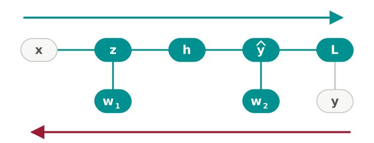
In the diagram, the gray pills are the given data \(x\) and \(y\), the teal pills are the computed values (the pre-activation \(z\), the hidden activation \(h\), the prediction \(\hat y\), the loss \(\mathcal{L}\)) and the parameters \(w_1\) and \(w_2\), entering where they multiply; the teal arrow is the forward pass and the cardinal arrow is the backward pass, running the same edges in reverse.

Automatic differentiation (autodiff) is the observation that the graph is enough. Each node applies one elementary operation, and every elementary operation has a one-line local derivative with respect to its own inputs: a product node contributes the other factor, a ReLU node contributes \(\mathbb{1}[z > 0]\), a squaring node contributes twice its input. The multivariate chain rule from last lecture then composes them into a gradient for the whole graph: \[ \frac{\partial \mathcal{L}}{\partial u} = \sum_{v} \frac{\partial \mathcal{L}}{\partial v}\cdot\frac{\partial v}{\partial u}, \] where the sum runs over the nodes \(v\) that \(u\) feeds directly. Nothing in that rule mentions the architecture, so nothing in it has to be re-derived when the architecture changes.

The direction of the sweep is what makes this cheap. Going backward, from \(\mathcal{L}\) toward the parameters, visits each node and edge once and produces the derivative of the one loss with respect to every node in the graph, where going forward, nudging one weight at a time as in last lecture’s comparison, would have to be repeated once per parameter.

Autodiff removes the labor from computing a gradient. It does nothing at all about the size of the sum sitting inside that gradient.

Stochastic Gradient Descent

Recall the shape of every loss we have written this semester, an average over data points with one term per example: \[ \mathcal{L}(\mathbf{w}) = \frac{1}{n}\sum_{i=1}^n \mathcal{L}_i(\mathbf{w}), \] where \(\mathcal{L}_i\) is the loss on example \(i\) alone. Its gradient inherits the same shape, so name the term belonging to one example the per-example gradient: \[ \mathbf{g}^{(i)} = \nabla_\mathbf{w}\mathcal{L}_i(\mathbf{w}) \in \mathbb{R}^d, \qquad \nabla_\mathbf{w}\mathcal{L}(\mathbf{w}) = \frac{1}{n}\sum_{i=1}^n \mathbf{g}^{(i)} . \] The full gradient is an average of \(n\) vectors, and Unit 1 spent an entire lecture on what to do with an average too expensive to compute exactly: sample it.

Draw a uniformly random batch of indices \(S \subseteq \{1,\ldots,n\}\) of size \(B\) and average over the batch alone: \[ \hat{\mathbf{g}}^{\mathrm{batch}} = \frac{1}{B}\sum_{i \in S}\mathbf{g}^{(i)} \in \mathbb{R}^d . \] Stepping along \(-\hat{\mathbf{g}}^{\mathrm{batch}}\) in place of the full gradient is stochastic gradient descent (SGD): \[ \mathbf{w}^{(t+1)} = \mathbf{w}^{(t)} - \alpha\, \hat{\mathbf{g}}^{\mathrm{batch}} . \] The hat is deliberate: this is an estimator of the full gradient in exactly the sense of the Monte Carlo lecture, so ask the two questions we asked of the sample mean \(\hat\mu_n\) there: is it right on average, and how far off is it typically?

The first one was our in-class exercise.

Claim: For a uniformly random batch \(S\) of size \(B\) drawn without replacement, the minibatch gradient is an unbiased estimator of the full gradient: \[ \mathbb{E}_S\big[\hat{\mathbf{g}}^{\mathrm{batch}}\big] = \nabla_\mathbf{w}\mathcal{L}(\mathbf{w}). \]

Proof of Claim

Rewrite the batch average as a sum over all \(n\) examples, with an indicator deciding which ones are present: \[ \hat{\mathbf{g}}^{\mathrm{batch}} = \frac{1}{B}\sum_{i=1}^n \mathbb{1}[i \in S]\,\mathbf{g}^{(i)} . \] Every index is equally likely to land in a uniformly random batch of size \(B\), so \(\Pr(i \in S) = B/n\) for every \(i\), and the expectation of an indicator is the probability of its event. Now take expectations, one move per equality: \[ \begin{align*} \mathbb{E}_S\big[\hat{\mathbf{g}}^{\mathrm{batch}}\big] &= \frac{1}{B}\sum_{i=1}^n \mathbb{E}_S\big[\mathbb{1}[i\in S]\big]\,\mathbf{g}^{(i)} \\&= \frac{1}{B}\sum_{i=1}^n \frac{B}{n}\,\mathbf{g}^{(i)} \\&= \frac{1}{n}\sum_{i=1}^n \mathbf{g}^{(i)} = \nabla_\mathbf{w}\mathcal{L}(\mathbf{w}). \end{align*} \] The first equality is linearity of expectation, which moves it inside the sum and past the fixed vectors \(\mathbf{g}^{(i)}\); the second substitutes \(\Pr(i \in S) = B/n\); the third cancels the \(B\). Notice what the argument never used: independence between the examples that land in a batch. Linearity of expectation holds regardless of how they relate, which is the same remark we made about \(\hat\mu_n\) in Unit 1.

This is the Monte Carlo estimator with a vector in place of a scalar: the full gradient is the unknown mean \(\mu\), one example’s gradient is a single sampled score, and the batch is the sample. So every theorem Unit 1 proved about sample means is already a theorem about training.

But being right on average is a low bar. The question that decides whether SGD is usable is the second one: how far does \(\hat{\mathbf{g}}^{\mathrm{batch}}\) typically sit from the gradient it is estimating?

Batch Size, Variance, and the Learning Rate

Let \(\sigma^2\), the gradient noise, measure how much a single example’s gradient disagrees with the full gradient, averaged over the dataset: \[ \sigma^2 = \frac{1}{n}\sum_{i=1}^n\big\|\mathbf{g}^{(i)} - \nabla_\mathbf{w}\mathcal{L}(\mathbf{w})\big\|_2^2 . \] It is large exactly when different examples pull the weights in different directions. Averaging a batch of \(B\) of those disagreements shrinks the expected squared error of the estimate: \[ \mathbb{E}_S\Big[\big\|\hat{\mathbf{g}}^{\mathrm{batch}} - \nabla_\mathbf{w}\mathcal{L}(\mathbf{w})\big\|_2^2\Big] \approx \frac{\sigma^2}{B} . \] That is the Monte Carlo lecture’s rate for \(\mathrm{Var}(\hat\mu_n)\) with \(B\) in place of \(n\): the typical error of one batch gradient is \(\sigma/\sqrt{B}\), so halving it costs four times the batch. Problem 12 derives this rate from the definition in a couple of lines, and then breaks it: when a dataset holds many near-duplicate examples their per-example gradients are correlated, and the correlation floor from Problem 1 caps how much any batch size can help.

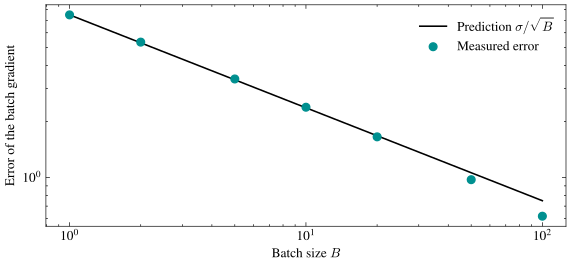
In the plot, the teal dots are the measured error \(\|\hat{\mathbf{g}}^{\mathrm{batch}} - \nabla_\mathbf{w}\mathcal{L}(\mathbf{w})\|_2\) of a batch gradient, and the black line is the predicted \(\sigma/\sqrt{B}\): on log-log axes, the straight line of slope \(-\frac12\) from Unit 1’s advantage roll.

Now put the two costs side by side. One batch gradient costs \(O(Bd)\) rather than \(O(nd)\), so for the compute of a single full-batch step we can take \(n/B\) stochastic ones: the number of affordable steps scales like \(1/B\) while the error of each scales only like \(1/\sqrt{B}\). That mismatch of exponents is the argument for SGD, since shrinking the batch buys steps faster than it costs accuracy.

The argument reverses near the minimum. There the full gradient goes to zero but \(\sigma^2\) does not, since individual examples still disagree about where the bottom is, so the update \(-\alpha\hat{\mathbf{g}}^{\mathrm{batch}}\) becomes a random step of length roughly \(\alpha\sigma/\sqrt{B}\). SGD does not converge to the minimum at all. It settles into a ball whose radius grows with \(\alpha\) and shrinks with \(\sqrt{B}\), and the demo plots exactly this: the full-batch run’s distance to the minimum keeps dropping while the stochastic runs flatten out at a floor.

There are two ways to lower that floor. Enlarging \(B\) costs arithmetic at every step for the rest of training. Shrinking \(\alpha\) costs nothing.

Learning Rate Schedules

A learning rate schedule makes the learning rate a function of the step count instead of a constant: \[ \alpha^{(t)} = \frac{\alpha^{(0)}}{1 + t/\tau}, \] where \(\alpha^{(0)} > 0\) is the starting learning rate and \(\tau > 0\) is the step count at which it has fallen to half of that. Early, when the true gradient dwarfs the noise, \(\alpha^{(t)} \approx \alpha^{(0)}\) and the steps are long; late, when the gradient is mostly noise, \(\alpha^{(t)}\) has shrunk and the noise ball closes in along with it. A schedule gets the small final error of a small learning rate without the slow start, which no constant \(\alpha\) can do.

(In practice the decay curve is chosen empirically, usually linear or cosine decay toward zero, often preceded by a short warmup that ramps \(\alpha\) up so early, badly-scaled gradients do not fling the weights somewhere useless.)

A schedule attacks the noise inside a step. It leaves the shape of the bowl exactly as the Optimization lecture found it.

Momentum

Recall that shape: writing \(\lambda_{\max}\) and \(\lambda_{\min}\) for the largest and smallest curvature of the loss, the Optimization lecture showed that gradient descent’s trouble is governed by their ratio: \[ \kappa = \frac{\lambda_{\max}}{\lambda_{\min}} . \] A step size small enough not to overshoot the steep direction is far too small for the shallow one, so the path zig-zags across the valley and the error contracts by only \(\frac{\kappa - 1}{\kappa + 1}\) per step.

The mechanical fix starts from noticing that the zig-zag is self-cancelling: across the valley the gradient alternates sign, while along the valley it points the same way every step, so averaging the gradients over time cancels the alternating part and keeps the consistent one. Momentum does exactly that. Write \(\hat{\mathbf{g}}^{(t)}\) for the batch gradient at step \(t\), and keep a running velocity \(\mathbf{v}^{(t)} \in \mathbb{R}^d\): \[ \mathbf{v}^{(t+1)} = \beta\,\mathbf{v}^{(t)} + \hat{\mathbf{g}}^{(t)}, \qquad \mathbf{w}^{(t+1)} = \mathbf{w}^{(t)} - \alpha\,\mathbf{v}^{(t+1)}, \] where \(\mathbf{v}^{(0)} = \mathbf{0}\) and \(\beta \in [0,1)\) (often \(0.9\)) sets how much of the previous velocity survives. Physically it is a ball rolling downhill: a new push changes its velocity but does not erase the speed it already had.

Unrolling the recurrence says precisely what the velocity is; substitute its definition into itself until the chain reaches \(\mathbf{v}^{(0)} = \mathbf{0}\): \[ \begin{align*} \mathbf{v}^{(t+1)} &= \hat{\mathbf{g}}^{(t)} + \beta\,\mathbf{v}^{(t)} \\&= \hat{\mathbf{g}}^{(t)} + \beta\,\hat{\mathbf{g}}^{(t-1)} + \beta^2\,\mathbf{v}^{(t-1)} \\&= \hat{\mathbf{g}}^{(t)} + \beta\,\hat{\mathbf{g}}^{(t-1)} + \beta^2\,\hat{\mathbf{g}}^{(t-2)} + \beta^3\,\mathbf{v}^{(t-2)} \\&= \sum_{k=0}^{t}\beta^k\,\hat{\mathbf{g}}^{(t-k)} . \end{align*} \] So the velocity is a weighted average of every gradient so far, with weights decaying geometrically into the past. The weights sum to nearly \(\frac{1}{1-\beta}\), which is \(10\) at \(\beta = 0.9\), so momentum’s effective step is about ten times what the same \(\alpha\) would give plain SGD, and raising \(\beta\) means lowering \(\alpha\). And averaging several noisy gradients reduces noise, exactly as averaging several samples did in Unit 1, which is Problem 12’s Part C: momentum trades a little bias for a lower-variance gradient estimate, biased because the gradients being averaged were measured at older weights. If you raised \(\beta\) from \(0.9\) to \(0.99\) and wanted the effective step to stay where it was, what would \(\alpha\) have to become?

Let’s take one real step, as we will at the board, on the univariate quadratic of curvature \(\lambda\): \[ \mathcal{L}(w) = \tfrac{\lambda}{2}w^2, \qquad \nabla_w\mathcal{L}(w) = \lambda w . \] Set \(\lambda = 1\), learning rate \(\alpha = 0.3\), momentum \(\beta = 0.8\), and starting point \(w^{(0)} = 4\). The first step is identical for both methods, because \(v^{(0)} = 0\) leaves momentum nothing to remember: \[ v^{(1)} = 0.8\cdot 0 + 4 = 4, \qquad w^{(1)} = 4 - 0.3\cdot 4 = 2.8 . \] The second step is where they separate, since plain gradient descent takes another ordinary step from \(w^{(1)} = 2.8\) while momentum adds the remembered velocity first: \[ w^{(2)}_{\text{gd}} = 2.8 - 0.3\cdot 2.8 = 1.96, \qquad v^{(2)} = 0.8\cdot 4 + 2.8 = 6.0, \qquad w^{(2)}_{\text{mom}} = 2.8 - 0.3\cdot 6.0 = 1.0 . \]

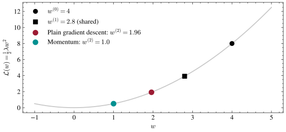
In the plot, the black circle and square mark the shared start and first step, and the two colored points are where the second step lands. Momentum ends at \(1.0\) against plain gradient descent’s \(1.96\), twice as close to the minimum after the same two gradient evaluations. One dimension has no zig-zag to cancel, so this example isolates momentum’s other half: the accumulated velocity lets it take a long step once several gradients in a row have agreed on a direction.

In more than one dimension both halves act at once, and the improvement can be stated exactly. Eliminating \(\mathbf{v}\) turns the two update rules into a single two-term recurrence in \(\mathbf{w}\), and tracking that recurrence’s roots gives the per-step contraction of momentum with well-chosen \(\alpha\) and \(\beta\): \[ \frac{\sqrt{\kappa} - 1}{\sqrt{\kappa} + 1} \qquad\text{against}\qquad \frac{\kappa-1}{\kappa+1} \quad\text{for plain gradient descent.} \] At the \(\kappa = 15\) of the demo’s bowl that is \(0.59\) against \(0.88\) per step. Momentum replaces the condition number with its square root, and Problem 12’s starred part derives that rate from the recurrence.

Momentum smooths the direction of a step. It still applies one \(\alpha\) to every parameter, and the whole trouble with \(\kappa\) was that one number has to serve directions of wildly different curvature.

Adaptive Methods

The last family adapts the size of the step per parameter, using gradient history as a stand-in for curvature: a consistently large gradient marks a steep direction that should take small steps, and a consistently small one marks a shallow direction that should take large steps.

Adagrad accumulates the squared gradients of each parameter \(j\) and divides that parameter’s step by the square root of the total: \[ s_j^{(t)} = \sum_{r=1}^{t}\big(\hat g_j^{(r)}\big)^2, \qquad w_j^{(t+1)} = w_j^{(t)} - \frac{\alpha}{\sqrt{s_j^{(t)}} + \epsilon}\,\hat g_j^{(t)}, \] where \(\hat g_j^{(t)}\) is coordinate \(j\) of the batch gradient at step \(t\) and \(\epsilon\) (around \(10^{-8}\)) keeps the denominator away from zero. The flaw is visible in the formula: \(s_j^{(t)}\) is a sum of squares, so it only ever grows, and the effective learning rate decays toward zero whether or not training is anywhere near finished.

RMSProp replaces that running sum with an exponential moving average, the same construction as momentum’s velocity applied to squared gradients: \[ s_j^{(t)} = \beta_2\, s_j^{(t-1)} + (1-\beta_2)\big(\hat g_j^{(t)}\big)^2 , \] with \(\beta_2\) close to \(1\). Old gradients are now forgotten geometrically rather than accumulated forever, so a direction that goes quiet can have its step size grow back.

Adam (Kingma and Ba) runs both averages at once: \[ v_j^{(t)} = \beta_1 v_j^{(t-1)} + (1-\beta_1)\hat g_j^{(t)}, \qquad s_j^{(t)} = \beta_2 s_j^{(t-1)} + (1-\beta_2)\big(\hat g_j^{(t)}\big)^2 , \] with \(\beta_1 = 0.9\) and \(\beta_2 = 0.999\) as the usual defaults. The step then divides momentum’s smoothed direction by RMSProp’s per-parameter scale: \[ w_j^{(t+1)} = w_j^{(t)} - \alpha\,\frac{v_j^{(t)} / (1-\beta_1^t)}{\sqrt{s_j^{(t)} / (1-\beta_2^t)} + \epsilon} . \] Both averages start at zero, so early steps are biased toward zero; dividing by \(1 - \beta_1^t\) and \(1 - \beta_2^t\), the weights actually used so far, rescales them back into honest averages. That bias correction is the same normalization Problem 12’s Part C applies to momentum before comparing its variance to a single batch gradient’s.

The class demo runs gradient descent, SGD, and Adam on this same stretched bowl built out of data, and its last cell raises the batch size live to watch the noise floor drop. Adam’s path stays smooth where gradient descent and SGD zig-zag, because adaptivity fixes the shape of the bowl. The noise inside each step is untouched, and only a smaller learning rate or a larger batch lowers it.

Looking Forward

One loose thread from last lecture’s hand computation is still hanging: a dead ReLU zeroed out an entire gradient path, and that was not an accident of the numbers we chose. Next lecture asks what happens when a network is fifty layers deep instead of two: the same phenomenon, compounded layer by layer, decided for decades whether deep networks could be trained at all.

If you carry one sentence out of today, carry this one: once a gradient is an average over data it is an estimator, so every question you would ask about an estimator (is it unbiased, how large is its variance, can averaging shrink it) is a question about training.