Generalization
The Methodology lecture gave us a picture we have leaned on ever since: bias falls and variance rises as a model gains capacity, and their sum traces a U that bottoms out before the model can fit the training data exactly. The Linear Model lecture planted a question we deferred twice: when a model has more parameters than data points, infinitely many hypotheses fit the training data exactly, so which one do our algorithms actually find? Today both threads finish, and they turn out to be the same thread.
A model with capacity to spare has many perfect fits, and how it generalizes depends on which one it picks. That preference comes from two places: a prior we write into the loss on purpose, and the optimizer itself, which prefers one fit over the others without being asked.
Regularization as a Prior
Start with the preference we choose on purpose. Handing a model fewer parameters is one way to ask for simplicity; this section builds a second that never touches the parameter count. Maximum likelihood, since the Mean Squared Error lecture, has picked the weights that make the data most probable. Maximum a posteriori (MAP) estimation adds a belief about the weights themselves, using Bayes’ rule from Unit 1: \[ \Pr(\mathbf{w} \mid \text{data}) \propto \Pr(\text{data} \mid \mathbf{w}) \cdot \Pr(\mathbf{w}). \] The prior is where “simpler” enters: the simplest belief about a weight vector \(\mathbf{w} \in \mathbb{R}^d\) is that its entries are small and centered at zero.
Claim: Under a Gaussian prior \(\mathbf{w} \sim \mathcal{N}(\mathbf{0}, \tau^2 \mathbf{I})\), where \(\tau^2 > 0\) is the prior variance of each weight, and the Gaussian noise model of the Mean Squared Error lecture, maximizing the posterior is equivalent to minimizing mean squared error plus a penalty on the weights’ squared length, \(\mathcal{L}(\mathbf{w}) + \lambda\|\mathbf{w}\|_2^2\), with strength \(\lambda = \sigma^2/(n\tau^2)\).
Proof of Claim
Take logs of both sides of Bayes’ rule, dropping the normalizing constant, which does not depend on \(\mathbf{w}\): \[ \log \Pr(\mathbf{w}\mid\text{data}) = \log \Pr(\text{data}\mid\mathbf{w}) + \log \Pr(\mathbf{w}) + \text{const}. \] The Mean Squared Error lecture already computed the first term for a hypothesis \(f\) with weights \(\mathbf{w}\) and Gaussian noise of variance \(\sigma^2\): \[ \log\Pr(\text{data}\mid\mathbf{w}) = -\frac{1}{2\sigma^2}\sum_{i=1}^n\big(y^{(i)}-f(\mathbf{x}^{(i)})\big)^2 + \text{const}. \] The second term is that same Gaussian density formula applied to \(\mathbf{w}\) instead of the noise, with \(\tau^2\) in place of \(\sigma^2\). The prior treats the \(d\) coordinates of \(\mathbf{w}\) as independent, so their densities multiply and the logarithm turns that product into a sum of squares: \[ \log\Pr(\mathbf{w}) = -\sum_{j=1}^d \frac{w_j^2}{2\tau^2} + \text{const} = -\frac{1}{2\tau^2}\|\mathbf{w}\|_2^2 + \text{const}. \] Add the two and negate, since maximizing the posterior is the same as minimizing its negative: \[ \arg\max_\mathbf{w} \log\Pr(\mathbf{w}\mid\text{data}) = \arg\min_\mathbf{w} \left[\frac{1}{2\sigma^2}\sum_{i=1}^n\big(y^{(i)}-f(\mathbf{x}^{(i)})\big)^2 + \frac{1}{2\tau^2}\|\mathbf{w}\|_2^2\right]. \] Multiplying through by the positive constant \(2\sigma^2/n\) leaves the minimizer alone and turns the first term into the mean squared error \(\mathcal{L}(\mathbf{w}) = \frac1n\sum_i (y^{(i)} - f(\mathbf{x}^{(i)}))^2\): \[ \arg\min_\mathbf{w} \left[\mathcal{L}(\mathbf{w}) + \lambda\|\mathbf{w}\|_2^2\right], \qquad \lambda = \frac{\sigma^2}{n\tau^2}. \]The regularization strength \(\lambda\) is large when the noise variance \(\sigma^2\) is large (unreliable labels, so lean on the prior), when the prior variance \(\tau^2\) is small (a firm belief that weights are small), and when \(n\) is small. That last dependence is the one to remember: a prior is a belief held before seeing data, and every data point dilutes it, so the penalty fades as the dataset grows.
This is ridge regression, and in the gradient-descent form of the Gradient Descent lecture it is weight decay, since the penalty’s gradient \(2\lambda\mathbf{w}\) shrinks every weight toward zero at each step. Swap the Gaussian prior for a Laplace prior on each weight and the identical recipe produces an \(\ell_1\) penalty \(\lambda\|\mathbf{w}\|_1\) instead of \(\ell_2\), which is lasso. The Laplace density carries \(|w_j|\) in its exponent rather than \(w_j^2\), so the log-prior penalty keeps a constant slope right up to zero instead of flattening out there, and a coordinate whose evidence is weaker than that slope is pushed to exactly zero: \(\ell_1\) produces genuinely sparse weight vectors and \(\ell_2\) does not. Choosing a penalty is choosing a prior, just as the Mean Squared Error lecture showed that choosing a loss is choosing a noise model; the maximum-likelihood thread that started there finishes with the policy gradient in the final unit.
A penalty is a preference we choose, tune on a validation set, and can always turn off; the rest of the lecture is about one we cannot. To see why that matters, first recall what the classical picture predicts.
The Classical U-Curve
Recall the decomposition the Methodology lecture built. Treat the training set itself as random, refit on each draw, and the expected squared error of the fitted hypothesis \(\hat f\) at a test point splits into three pieces: \[ \mathbb{E}\big[(y - \hat f(x))^2\big] = \underbrace{\big(\mathbb{E}[\hat f(x)] - f^*(x)\big)^2}_{\text{bias}^2} + \underbrace{\mathrm{Var}(\hat f(x))}_{\text{variance}} + \underbrace{\mathrm{Var}(y \mid x)}_{\text{noise}} . \] Bias is how far the average fit sits from the truth \(f^*\), variance is how much the fit swings from one training set to the next, and the noise term is the floor no model beats. As capacity grows, bias falls and variance rises, since a richer class can bend closer to the truth but has more room to chase this training set’s noise, and their sum traces the U.
Keep the number of training points \(n\) fixed and let \(d\) be the number of features the model uses, so the design matrix is \(\mathbf{X}\in\mathbb{R}^{n\times d}\). The Methodology lecture called \(d = n\) the interpolation threshold: there the model has exactly enough freedom to hit every training label, and training error drops to zero. Every model on the classical U sits to the left of that line, and the U-curve’s verdict on the other side is an extrapolation of the variance term: more capacity, more room to chase noise, more error, forever. Testing that extrapolation means building models with \(d > n\), the question the Linear Model lecture left open.
Which Interpolating Solution Do We Find?
When \(d > n\), the design matrix has more columns than rows and \(\mathbf{X}\mathbf{w}=\mathbf{y}\) has a whole subspace of exact solutions; all have zero training error, so the training loss cannot choose between them, and yet they generalize very differently. Gradient descent started from \(\mathbf{w}^{(0)}=\mathbf{0}\) and the closed-form pseudoinverse both return the same weights \(\hat{\mathbf{w}} \in \mathbb{R}^d\), the minimum-norm solution: \[ \hat{\mathbf{w}} = \arg\min\big\{\|\mathbf{w}\|_2 \;:\; \mathbf{X}\mathbf{w}=\mathbf{y}\big\} . \]
Let’s find one by hand, exactly as we will in class. Take the single equation \(w_1 + 2w_2 = 3\): one equation in two unknowns, with an entire line of exact solutions.
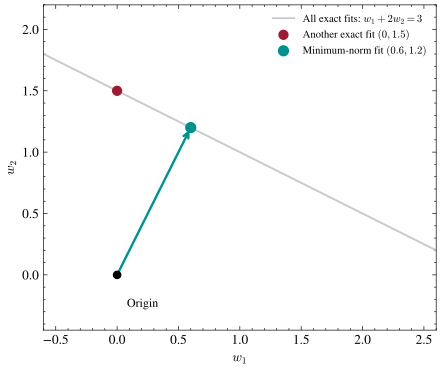
In the plot, the gray line is the set of exact fits, and the minimum-norm solution is the point on it closest to the origin, found the same way the Linear Model lecture found a projection: drop a perpendicular from \(\mathbf{0}\) onto the line. Write the constraint as \(\mathbf{a}^\top\mathbf{w}=3\) for \(\mathbf{a}=(1,2)\), and the foot of that perpendicular is: \[ \hat{\mathbf{w}} = \mathbf{a}\,(\mathbf{a}^\top\mathbf{a})^{-1}\cdot 3 = \frac{3}{1^2 + 2^2}\,(1,2) = \tfrac{3}{5}(1,2) = (0.6,\, 1.2) . \] It satisfies the constraint, since \(0.6 + 2.4 = 3\), and its norm \(\sqrt{0.6^2 + 1.2^2} = \sqrt{1.8} \approx 1.34\) is smaller than that of the equally exact fit \((0, 1.5)\), drawn in cardinal, whose norm is \(1.5\). That formula is the pseudoinverse from the Optimization lecture, applied to an underdetermined system: \(\hat{\mathbf{w}} = \mathbf{X}^+\mathbf{y}\), the same expression that solved least squares, now selecting the minimum-norm solution instead of the closest-fit one.
Nobody told gradient descent to prefer small weights here: there is no penalty and no prior, so the preference has to come from the shape of the steps themselves.
Claim: Gradient descent on mean squared error, started at \(\mathbf{w}^{(0)}=\mathbf{0}\), keeps every iterate in the span of the data points \(\mathbf{x}^{(1)},\ldots,\mathbf{x}^{(n)}\) (the row space of \(\mathbf{X}\)).
Proof of Claim
The Optimization lecture computed the gradient of the mean squared error of a linear model. Writing \(\mathbf{r} = \mathbf{X}\mathbf{w} - \mathbf{y} \in \mathbb{R}^n\) for the residual vector, whose \(i\)th entry \(r^{(i)}\) is the error on data point \(i\), that gradient expands as a combination of the data points: \[ \nabla_\mathbf{w}\mathcal{L}(\mathbf{w}) = \frac{2}{n}\mathbf{X}^\top(\mathbf{X}\mathbf{w}-\mathbf{y}) = \frac{2}{n}\mathbf{X}^\top\mathbf{r} = \frac{2}{n}\sum_{i=1}^n r^{(i)}\,\mathbf{x}^{(i)}, \] where the last equality is the outer-product view of a matrix-vector product: \(\mathbf{X}^\top\) has the data points as its columns, so \(\mathbf{X}^\top\mathbf{r}\) weights each data point by its own residual and adds them up. Now induct on \(t\). The start \(\mathbf{w}^{(0)} = \mathbf{0}\) is in the span, and if \(\mathbf{w}^{(t)}\) is in the span then so is \(\mathbf{w}^{(t+1)} = \mathbf{w}^{(t)} - \alpha\nabla_\mathbf{w}\mathcal{L}(\mathbf{w}^{(t)})\), because we subtracted one more combination of the same \(n\) vectors.Now compare that against the set of exact fits. Moving from one exact fit to another means adding a vector \(\mathbf{z}\) with \(\mathbf{X}\mathbf{z}=\mathbf{0}\), which says \(\langle\mathbf{x}^{(i)}, \mathbf{z}\rangle = 0\) for every data point: the freedom the training loss leaves us runs perpendicular to the span gradient descent is confined to. The \(n\)-dimensional span therefore meets the \((d-n)\)-dimensional set of exact fits in exactly one point, and Problem 14 shows that point is the minimum-norm solution. Stochastic gradient descent inherits the whole argument, since a minibatch gradient is a combination of a subset of the same data points. This is implicit regularization: the optimizer’s own trajectory, rather than a term added to the loss, decides which of infinitely many perfect fits we end up with.
This preference comes free, and it is the same one a Gaussian prior would have expressed. At one particular model size, though, it goes badly wrong.
The Interpolation Threshold Is a Conditioning Catastrophe
Push the model-size dial past the interpolation threshold: keep the true signal confined to a handful of the \(d\) features, treat the rest as pure noise, and grow \(d\) toward \(n\) and well past it, refitting the minimum-norm solution at each size. The test error does something strange: it spikes right at \(d = n\), far above the error on either side, then falls again as \(d\) grows further. The class demo runs exactly this sweep and watches the spike happen.
The spike should bother you: a model past the threshold fits the training set exactly no matter how many more features we hand it, so it is not obvious why the number of surplus parameters should change anything. The answer is that these models interpolate with wildly different weights, and the size of those weights is set by the geometry of \(\mathbf{X}\).
The mechanism is the condition number from the Optimization lecture, applied to test error instead of to precision. Recall that the pseudoinverse builds the minimum-norm solution by inverting each singular value in place: \[ \mathbf{X}^+ = \sum_{i=1}^n \frac{1}{\sigma_i}\mathbf{v}_i\mathbf{u}_i^\top, \qquad \hat{\mathbf{w}} = \mathbf{X}^+\mathbf{y} , \] where \(\sigma_1 \geq \cdots \geq \sigma_n > 0\) are the singular values of \(\mathbf{X}\) (not the noise level \(\sigma^2\) from the prior section), and \(\mathbf{u}_i \in \mathbb{R}^n\) and \(\mathbf{v}_i \in \mathbb{R}^d\) are its left and right singular vectors. A small singular value \(\sigma_i\) marks a direction along which the training features barely vary, so the data says almost nothing about the corresponding weight; dividing by it turns a small amount of label noise into an enormous coefficient in \(\hat{\mathbf{w}}\), which does its damage on test points where that direction does vary. A standard result for random matrices says where the smallest singular value lands when the entries of \(\mathbf{X}\) are independent standard Gaussians: \[ \sigma_{\min} \approx \big|\sqrt{d}-\sqrt{n}\big| . \] It vanishes exactly at \(d=n\) and grows steadily on either side, so the factor \(1/\sigma_{\min}\) that the pseudoinverse applies to the labels, and with it the condition number \(\kappa(\mathbf{X}) = \sigma_{\max}/\sigma_{\min}\), is largest precisely at the interpolation threshold.
Past the threshold, each new feature adds a fresh direction, the singular values lift away from zero, and the minimum-norm solution can spread one interpolating fit across many directions so that no single one carries an amplified coefficient. That is the second descent. It does not continue forever: the fit still lives in the span of the \(n\) data points, an \(n\)-dimensional slice of the \(\mathbb{R}^d\) that \(\mathbf{w}^*\) lives in, so it captures a fraction of the signal that shrinks like \(n/d\). Eventually the missed signal outweighs the falling noise, and the error drifts back up. The best model overall is still the small one that uses only the informative features; the second descent does not beat it, but it makes the very large models usable at all, instead of the disaster the U-curve’s extrapolation predicted. Problem 14 makes the whole shape exact: it splits \(\hat{\mathbf{w}}\) into a signal piece and a noise piece, measures the noise piece in terms of the singular values, and reads both the spike and the descent off that one formula.
This is double descent, and it overturns the assumption baked into the Methodology lecture’s U-curve. Past the interpolation threshold, more parameters need not mean worse generalization: it means a better-conditioned design matrix, and the variance term follows the conditioning rather than the parameter count.
Looking Forward
This closes the Neural Networks unit. Modern networks carry far more parameters than training points, so they live far out on the right side of this curve, and the conditioning story above is a large part of why that works at all.
The next unit asks what structure the weights and representations of a trained network actually have. The answer is low rank, and the tool is the SVD, which returns in the very next lecture as the best rank-\(k\) approximation of a matrix: instead of dividing by the smallest singular values, we ask what happens when we throw them away.
Carry one sentence out of today: once a model has more than one perfect fit available, the algorithm’s unstated preference among them decides which one we get, and the parameter count is a poor proxy for capacity.