Demo: Low-rank Approximation of an Image and a Video

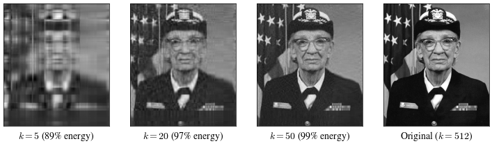
Same photograph as the Linear Algebra lecture’s warp demo, and the same theorem from today’s reading: truncate the SVD, keep the top \(k\) singular values, and see how little rank it actually takes to recognize a picture. Then we do the same thing to a video.

import numpy as np
import matplotlib.pyplot as plt
import matplotlib.cbook as cbook
import scienceplots

plt.style.use(["science", "no-latex"])
TEAL, CARDINAL, GRAY = "#009090", "#9c1b33", "#c9c9c9"

with cbook.get_sample_data("grace_hopper.jpg") as f:
    img = plt.imread(f)
gray = img.mean(axis=2)
u, s, vt = np.linalg.svd(gray, full_matrices=False)
print(f"image shape: {gray.shape}, {len(s)} singular values")

image shape: (600, 512), 512 singular values

def rank_k(u, s, vt, k):
    return (u[:, :k] * s[:k]) @ vt[:k, :]

total_energy = np.sum(s ** 2)
fig, axes = plt.subplots(1, 4, figsize=(9, 3))
for ax, k in zip(axes[:3], [5, 20, 50]):
    approx = rank_k(u, s, vt, k)
    captured = np.sum(s[:k] ** 2) / total_energy
    ax.imshow(approx, cmap="gray")
    ax.set_xlabel(f"$k={k}$ ({captured:.0%} energy)")
    ax.set_xticks([]); ax.set_yticks([])
axes[3].imshow(gray, cmap="gray")
axes[3].set_xlabel(f"Original ($k={len(s)}$)")
axes[3].set_xticks([]); axes[3].set_yticks([])
plt.show()

Why so few directions are enough

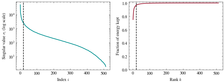
The reason \(k=20\) gets that close is the shape of the spectrum. On the left, the singular values on a log scale; on the right, the fraction of the energy \(\sum_i \sigma_i^2\) kept by a rank-\(k\) truncation. The dashed line marks \(k=20\) in both.

idx = np.arange(1, len(s) + 1)
cumulative = np.cumsum(s ** 2) / total_energy
n, d = gray.shape

fig, axes = plt.subplots(1, 2, figsize=(9, 3))
axes[0].plot(idx, s, color=TEAL, linewidth=1.6)
axes[0].axvline(20, color="black", linestyle="--", linewidth=1.2)
axes[0].set_yscale("log")
axes[0].set_xlabel("Index $i$")
axes[0].set_ylabel("Singular value $\\sigma_i$ (log scale)")

axes[1].plot(idx, cumulative, color=CARDINAL, linewidth=1.6)
axes[1].axvline(20, color="black", linestyle="--", linewidth=1.2)
axes[1].set_ylim(0, 1.02)
axes[1].set_xlabel("Rank $k$")
axes[1].set_ylabel("Fraction of energy kept")
plt.show()

print(f"rank 20 keeps {cumulative[19]:.0%} of the energy")
print(f"rank 20 costs {20 * (n + d + 1) / (n * d):.0%} of the storage")

rank 20 keeps 97% of the energy
rank 20 costs 7% of the storage

Now a video

Flatten every frame of a short video into one column of a big matrix (pixels \(\times\) frames); the SVD of that matrix tells us how many “directions” the whole video actually needs.

rng = np.random.default_rng(15)
T, H, W = 60, 40, 40
xs, ys = np.meshgrid(np.arange(W), np.arange(H))

frames = []
for t in range(T):
    cx = 5 + (W - 10) * t / (T - 1)   # a blob drifting left to right
    cy = H / 2
    frame = np.exp(-((xs - cx) ** 2 + (ys - cy) ** 2) / (2 * 6 ** 2))
    frame += rng.normal(0, 0.02, size=frame.shape)
    frames.append(frame.ravel())

M = np.array(frames).T   # (H*W) x T: one column per frame
print("video-as-matrix shape:", M.shape)

u_v, s_v, vt_v = np.linalg.svd(M, full_matrices=False)
total_v = np.sum(s_v ** 2)
for k in [1, 2, 3, 5]:
    print(f"rank {k}: {np.sum(s_v[:k] ** 2) / total_v:.1%} of the video's energy")

video-as-matrix shape: (1600, 60)
rank 1: 56.7% of the video's energy
rank 2: 86.2% of the video's energy
rank 3: 96.5% of the video's energy
rank 5: 99.4% of the video's energy

fig, axes = plt.subplots(2, 4, figsize=(9, 5))
frame_ids = [0, 20, 40, 59]
for col, t in enumerate(frame_ids):
    axes[0, col].imshow(frames[t].reshape(H, W), cmap="gray")
    axes[0, col].set_xlabel(f"Original, frame {t}")
    axes[0, col].set_xticks([]); axes[0, col].set_yticks([])

k = 3
M_k = rank_k(u_v, s_v, vt_v, k)
for col, t in enumerate(frame_ids):
    axes[1, col].imshow(M_k[:, t].reshape(H, W), cmap="gray")
    axes[1, col].set_xlabel(f"Rank-{k}, frame {t}")
    axes[1, col].set_xticks([]); axes[1, col].set_yticks([])
plt.show()

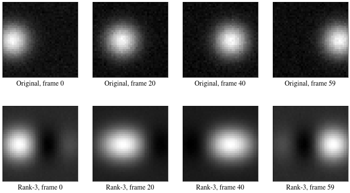
A single moving blob barely needs rank \(3\): almost the entire video is “the same frame, shifted,” and shifting is just a few singular directions’ worth of information.

What if the video were noisier?

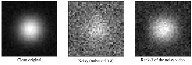
The reading’s denoising claim says a low-rank reconstruction should discard more noise than signal. Try noise_std = 0.3 below (much noisier than the 0.02 used above) and compare the rank-\(3\) reconstruction to the noisy original.

noise_std = 0.3    # change me!

frames_noisy = []
for t in range(T):
    cx = 5 + (W - 10) * t / (T - 1)
    cy = H / 2
    frame = np.exp(-((xs - cx) ** 2 + (ys - cy) ** 2) / (2 * 6 ** 2))
    frame += rng.normal(0, noise_std, size=frame.shape)
    frames_noisy.append(frame.ravel())

M_noisy = np.array(frames_noisy).T
u_n, s_n, vt_n = np.linalg.svd(M_noisy, full_matrices=False)
M_noisy_k = rank_k(u_n, s_n, vt_n, 3)

fig, axes = plt.subplots(1, 3, figsize=(8, 3))
t_show = 30
axes[0].imshow(frames[t_show].reshape(H, W), cmap="gray")
axes[0].set_xlabel("Clean original")
axes[1].imshow(frames_noisy[t_show].reshape(H, W), cmap="gray")
axes[1].set_xlabel(f"Noisy (noise std ${noise_std}$)")
axes[2].imshow(M_noisy_k[:, t_show].reshape(H, W), cmap="gray")
axes[2].set_xlabel("Rank-3 of the noisy video")
for ax in axes:
    ax.set_xticks([]); ax.set_yticks([])
plt.show()

Punchline: the rank-\(3\) reconstruction of the noisy video looks almost as clean as the original. The blob’s motion lives almost entirely in the top \(3\) singular directions while the noise spreads its energy thinly across all \(60\), so truncating throws away far more noise than signal. That is the reading’s denoising argument, now visible frame by frame.