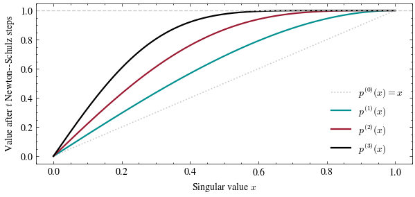
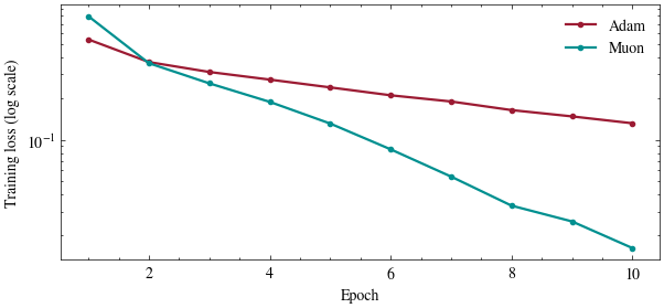
Muon orthogonalizes a gradient matrix \(\mathbf{G}\): it drives every singular value to \(1\) and leaves the singular vectors alone, using nothing but matrix multiplications. First we watch the Newton–Schulz cubic \(p(x) = (3x - x^3)/2\) turn into a step function one iteration at a time. Then we train a real network two ways, with Adam and with Muon, and compare.
import numpy as npimport matplotlib.pyplot as pltimport scienceplotsimport torchimport torch.nn as nnfrom sklearn.datasets import fetch_openmlplt.style.use(["science", "no-latex"])TEAL, CARDINAL, GRAY ="#009090", "#9c1b33", "#c9c9c9"def p(x):return (3* x - x **3) /2x = np.linspace(0, 1, 400)fig, ax = plt.subplots(figsize=(7, 3))ax.plot(x, x, color=GRAY, linewidth=1.2, linestyle=":", label="$p^{(0)}(x) = x$")iterate = x.copy()for i, color inzip(range(1, 4), [TEAL, CARDINAL, "black"]): iterate = p(iterate) ax.plot(x, iterate, color=color, linewidth=1.6, label=f"$p^{{({i})}}(x)$")ax.axhline(1.0, color=GRAY, linewidth=1.0, linestyle="--")ax.set_xlabel("Singular value $x$")ax.set_ylabel("Value after $t$ Newton--Schulz steps")ax.legend(frameon=False, loc="lower right")plt.show()
Three iterations already lift everything above \(x \approx 0.5\) to within a few percent of \(1\), which is sign(x) for \(x > 0\).
The reading’s claim says that applying this cubic to a matrix, as \(\tfrac32\mathbf{X} - \tfrac12\mathbf{X}\mathbf{X}^\top\mathbf{X}\), applies \(p\) to each singular value on its own. Let’s check that on the same matrix the reading’s spectrum figure plots.
rng = np.random.default_rng(18)G = rng.standard_normal((12, 12))Gt = G / np.linalg.norm(G, 2) # rescale so the largest singular value is exactly 1before = np.linalg.svd(Gt, compute_uv=False)for _ inrange(5): Gt =1.5* Gt -0.5* Gt @ Gt.T @ Gt # one Newton-Schulz step: two matrix multiplicationsafter = np.linalg.svd(Gt, compute_uv=False)print("rescaled singular values of G:", np.round(before, 3))print("after 5 Newton-Schulz steps: ", np.round(after, 3))print(f"smallest: {before[-1]:.3f} before, {after[-1]:.3f} after")
Every singular value moved up, the top ones are pinned at \(1\), and the smallest is still the laggard at \(0.196\): five steps is not enough for a badly conditioned matrix. That is the interval \([\ell, 1]\) from the reading. (Here we divided by the largest singular value, so the interval really does reach \(1\); the training loop below divides by the Frobenius norm instead, which costs one pass over the entries and still keeps every singular value at most \(1\).) Problem 18 works out how long that climb takes and where it ends up.
Muon vs. Adam on real data
Now train a small MLP on MNIST twice: once with Adam, once with Muon (momentum, orthogonalized by Newton–Schulz before every step). Nothing else changes.
torch.manual_seed(18)rng = np.random.default_rng(18)X, y = fetch_openml("mnist_784", version=1, return_X_y=True, as_frame=False, parser="auto")y = y.astype(int)idx = rng.choice(len(X), size=6000, replace=False)X, y = X[idx] /255.0, y[idx]n_train =5000Xtr_t = torch.tensor(X[:n_train], dtype=torch.float32)ytr_t = torch.tensor(y[:n_train], dtype=torch.long)Xte_t = torch.tensor(X[n_train:], dtype=torch.float32)yte_t = torch.tensor(y[n_train:], dtype=torch.long)class MLP(nn.Module):def__init__(self):super().__init__()self.fc1 = nn.Linear(784, 256)self.fc2 = nn.Linear(256, 10)def forward(self, x):returnself.fc2(torch.relu(self.fc1(x)))def newton_schulz(M, steps=5): Z = M / (M.norm() +1e-7) # Frobenius norm, so every singular value is at most 1for _ inrange(steps): Z =1.5* Z -0.5* Z @ Z.T @ Zreturn Z
def train(use_muon, epochs=10, lr=1e-3, muon_lr=0.02, beta=0.9): model = MLP() lossfn = nn.CrossEntropyLoss()ifnot use_muon: opt = torch.optim.Adam(model.parameters(), lr=lr) momentum = {prm: torch.zeros_like(prm) for prm in model.parameters()} losses = []for epoch inrange(epochs): perm = torch.randperm(len(Xtr_t))for i inrange(0, len(Xtr_t), 128): b = perm[i:i +128]for prm in model.parameters(): prm.grad =None loss = lossfn(model(Xtr_t[b]), ytr_t[b]) loss.backward()if use_muon:with torch.no_grad():for prm in model.parameters(): momentum[prm] = beta * momentum[prm] + prm.gradif prm.dim() ==2: # a weight matrix: orthogonalize prm -= muon_lr * newton_schulz(momentum[prm])else: # a bias vector: plain momentum prm -= lr * momentum[prm]else: opt.step()with torch.no_grad(): losses.append(lossfn(model(Xtr_t), ytr_t).item())with torch.no_grad(): acc = (model(Xte_t).argmax(1) == yte_t).float().mean().item()return losses, acclosses_adam, acc_adam = train(use_muon=False)losses_muon, acc_muon = train(use_muon=True)print(f"Adam: final training loss {losses_adam[-1]:.3f}, test accuracy {acc_adam:.1%}")print(f"Muon: final training loss {losses_muon[-1]:.3f}, test accuracy {acc_muon:.1%}")
Adam: final training loss 0.132, test accuracy 94.4%
Muon: final training loss 0.016, test accuracy 95.1%
Five Newton–Schulz steps do not reach the exact polar factor, as the spectrum above showed, and the run above says five is good enough anyway. Try ns_steps = 1 below. Does one step still beat Adam, or does Muon need several before the step is worth taking?
ns_steps =1# change me!def train_muon_custom(ns_steps, epochs=10, lr=1e-3, muon_lr=0.02, beta=0.9): model = MLP() lossfn = nn.CrossEntropyLoss() momentum = {prm: torch.zeros_like(prm) for prm in model.parameters()} losses = []for epoch inrange(epochs): perm = torch.randperm(len(Xtr_t))for i inrange(0, len(Xtr_t), 128): b = perm[i:i +128]for prm in model.parameters(): prm.grad =None loss = lossfn(model(Xtr_t[b]), ytr_t[b]) loss.backward()with torch.no_grad():for prm in model.parameters(): momentum[prm] = beta * momentum[prm] + prm.gradif prm.dim() ==2: prm -= muon_lr * newton_schulz(momentum[prm], ns_steps)else: prm -= lr * momentum[prm]with torch.no_grad(): losses.append(lossfn(model(Xtr_t), ytr_t).item())return losseslosses_custom = train_muon_custom(ns_steps)print(f"final training loss, Muon with {ns_steps} Newton-Schulz step(s): {losses_custom[-1]:.4f}")print(f"final training loss, Muon with 5 Newton-Schulz steps: {losses_muon[-1]:.4f}")print(f"final training loss, Adam: {losses_adam[-1]:.4f}")
final training loss, Muon with 1 Newton-Schulz step(s): 0.2049
final training loss, Muon with 5 Newton-Schulz steps: 0.0162
final training loss, Adam: 0.1319
Punchline: with one Newton–Schulz step the momentum is barely orthogonalized and Muon loses to Adam; with five it wins by a factor of eight on training loss. The network, the data, and the loss never changed, so all of that came from the direction of each step, bought with a handful of matrix multiplications.