Muon
Every optimizer we have built, from gradient descent through momentum to Adam, treats the parameters as one flat vector: a weight matrix \(\mathbf{W}\in\mathbb{R}^{d\times k}\) becomes a list of \(dk\) numbers before any update touches it. Last lecture accepted that reshaping and asked which entries we may move: LoRA froze \(\mathbf{W}\) and trained a rank-\(r\) correction. This closing lecture of the Low-Rank Structure unit keeps every entry trainable and asks whether the reshaping itself throws something away.
The answer turns on the word size. Gradient descent takes the fixed-size step that decreases the loss fastest, and a size is a norm; flattening commits us to one particular norm without mentioning it. Today we work out which norm a linear map deserves, which step is steepest under it, and why that step costs only a few matrix multiplications.
Steepest Descent Depends on the Norm
Recall the justification for the gradient direction from the Optimization lecture: among all steps of a fixed size, the negative gradient decreases the loss fastest. Let’s write that argument out for a matrix parameter to see exactly where the choice of size enters. Write \(\mathbf{G}\) for the gradient of the loss with respect to the weight matrix at the current weights: \[ \mathbf{G} = \nabla_\mathbf{W}\mathcal{L}(\mathbf{W}) \in \mathbb{R}^{d\times k} . \] It has one entry for each entry of \(\mathbf{W}\), so the first-order change in the loss caused by a step \(\mathbf{\Delta}\in\mathbb{R}^{d\times k}\) is the ordinary entrywise dot product of the two matrices: \[ \mathcal{L}(\mathbf{W}+\mathbf{\Delta}) \approx \mathcal{L}(\mathbf{W}) + \langle\mathbf{G},\mathbf{\Delta}\rangle , \quad\text{where}\quad \langle\mathbf{G},\mathbf{\Delta}\rangle = \sum_{i=1}^d\sum_{j=1}^k [\mathbf{G}]_{i,j}\,[\mathbf{\Delta}]_{i,j} . \] Steepest descent is now a small optimization problem of its own, with the learning rate \(\alpha>0\) as a budget on the step’s size: \[ \mathbf{\Delta} = \arg\min_{\|\mathbf{\Delta}\|\,\leq\,\alpha} \ \langle\mathbf{G},\mathbf{\Delta}\rangle . \] Everything depends on which norm \(\|\cdot\|\) sits in that constraint, and nothing above chooses it for us.
Flattening the matrix chooses the Frobenius norm, the Euclidean length of the \(dk\) entries laid out in a row: \[ \|\mathbf{M}\|_F = \sqrt{\sum_{i=1}^d\sum_{j=1}^k [\mathbf{M}]_{i,j}^2} = \sqrt{\sum_i\sigma_i^2} , \] where \(\sigma_1\geq\sigma_2\geq\cdots\) are the singular values of \(\mathbf{M}\) and the second equality is the identity from the Low-rank Approximation lecture. Under this budget, the Cauchy–Schwarz inequality applied to the two matrices read as vectors of length \(dk\) bounds how negative the inner product can get: \[ \langle\mathbf{G},\mathbf{\Delta}\rangle \ \geq\ -\|\mathbf{G}\|_F\,\|\mathbf{\Delta}\|_F \ \geq\ -\alpha\,\|\mathbf{G}\|_F , \] with equality exactly when \(\mathbf{\Delta}\) points opposite \(\mathbf{G}\) and spends the whole budget: \[ \mathbf{\Delta}^{\mathrm{frob}} = -\alpha\,\frac{\mathbf{G}}{\|\mathbf{G}\|_F} . \] That is plain gradient descent, with the learning rate absorbing the normalization, so every optimizer we have written down so far was solving this problem without saying so.
A linear map has a size of its own, independent of how its entries are stored: the largest factor by which it stretches a vector. That is the spectral norm from the Depth-enablers lecture, which the Decompositions lecture identified with the top singular value: \[ \|\mathbf{M}\|_2 = \max_{\mathbf{x}\neq\mathbf{0}}\frac{\|\mathbf{M}\mathbf{x}\|_2}{\|\mathbf{x}\|_2} = \sigma_1 . \] The Frobenius norm adds up the squares of every singular value; the spectral norm keeps only the largest. Spreading a step’s total movement evenly over fifty directions instead of one leaves its Frobenius norm unchanged but makes each singular value \(\sqrt{50}\) times smaller than the single value it replaced, so under the spectral norm the spread-out step costs about seven times less.
Which of the two should we be budgeting with? Ask what a change to \(\mathbf{W}\) does to the layer that contains it. The layer maps an input \(\mathbf{x}\in\mathbb{R}^k\) to \(\mathbf{W}\mathbf{x}\in\mathbb{R}^d\), so changing the weights by \(\mathbf{\Delta}\) moves that output by \[ \big\|(\mathbf{W}+\mathbf{\Delta})\mathbf{x} - \mathbf{W}\mathbf{x}\big\|_2 = \|\mathbf{\Delta}\mathbf{x}\|_2 \leq \|\mathbf{\Delta}\|_2\,\|\mathbf{x}\|_2 , \] where the inequality is the definition of the spectral norm. So a spectral-norm budget is a promise about the function the layer computes: no input’s output moves by more than \(\alpha\) times that input’s own length. A Frobenius budget makes no such promise, since it lets a step be small in total while still stretching one unlucky direction hard. That is the concern the Depth-enablers lecture raised about products of layer Jacobians, asked now about the update rather than the weights.
So which matrix is steepest under a spectral-norm budget? The SVD answers it.
The Optimal Update Is the Orthogonalized Gradient
Claim: Let \(\mathbf{G} = \mathbf{U}\mathbf{\Sigma}\mathbf{V}^\top = \sum_{i=1}^r \sigma_i\mathbf{u}_i\mathbf{v}_i^\top\) be the SVD of the gradient, with rank \(r\), orthonormal columns in \(\mathbf{U}\in\mathbb{R}^{d\times r}\) and \(\mathbf{V}\in\mathbb{R}^{k\times r}\), and the nonzero singular values on the diagonal of \(\mathbf{\Sigma}\in\mathbb{R}^{r\times r}\). Then the steepest-descent step under a spectral-norm budget of \(\alpha\) is \[ \mathbf{\Delta}^{\mathrm{spec}} = -\alpha\,\mathbf{U}\mathbf{V}^\top , \] and it decreases the linearized loss by \(\alpha\sum_{i=1}^r\sigma_i\).
Proof of Claim
Substitute the outer-product form of \(\mathbf{G}\) into the inner product and pull the sum out: \[ \begin{align*} \langle\mathbf{G},\mathbf{\Delta}\rangle &= \Big\langle \sum_{i=1}^r \sigma_i\mathbf{u}_i\mathbf{v}_i^\top,\ \mathbf{\Delta}\Big\rangle \\&= \sum_{i=1}^r \sigma_i\,\big\langle \mathbf{u}_i\mathbf{v}_i^\top,\ \mathbf{\Delta}\big\rangle \\&= \sum_{i=1}^r \sigma_i\ \mathbf{u}_i^\top\mathbf{\Delta}\mathbf{v}_i , \end{align*} \] where the second equality is linearity of the inner product and the third writes out the entrywise definition, \(\langle\mathbf{a}\mathbf{b}^\top,\mathbf{\Delta}\rangle = \sum_{i,j}a_ib_j[\mathbf{\Delta}]_{i,j} = \mathbf{a}^\top\mathbf{\Delta}\mathbf{b}\). Now bound one term at a time. Since \(\mathbf{u}_i\) and \(\mathbf{v}_i\) are unit vectors, \[ \big|\mathbf{u}_i^\top\mathbf{\Delta}\mathbf{v}_i\big| \leq \|\mathbf{u}_i\|_2\,\|\mathbf{\Delta}\mathbf{v}_i\|_2 \leq \|\mathbf{\Delta}\|_2 \leq \alpha , \] by Cauchy–Schwarz, then the definition of the spectral norm, then the budget. Every \(\sigma_i\) is nonnegative, so the whole sum cannot fall below \(-\alpha\sum_i\sigma_i\). It remains to exhibit a step that attains that value, and \(\mathbf{\Delta} = -\alpha\mathbf{U}\mathbf{V}^\top\) does. It is admissible: \(\mathbf{U}\mathbf{V}^\top\) sends each \(\mathbf{v}_i\) to the unit vector \(\mathbf{u}_i\) and sends everything orthogonal to all the \(\mathbf{v}_i\) to \(\mathbf{0}\), so it stretches no vector by more than \(1\) and \(\|\mathbf{\Delta}\|_2 = \alpha\). And it attains the bound, orthonormality gives \(\mathbf{u}_i^\top(\mathbf{U}\mathbf{V}^\top)\mathbf{v}_i = \mathbf{u}_i^\top\mathbf{u}_i = 1\) for every \(i\), so \(\langle\mathbf{G},\mathbf{\Delta}\rangle = -\alpha\sum_i\sigma_i\).The step keeps the gradient’s singular vectors and discards its singular values: every direction the gradient uses at all gets pushed exactly as hard as every other, and the directions it ignores, where \(\sigma_i = 0\), are not pushed at all. This matrix is the polar factor of \(\mathbf{G}\), and computing it is called orthogonalizing the gradient. Compare the two decreases we have derived, \(\alpha\sum_i\sigma_i\) for the orthogonalized step against \(\alpha\sqrt{\sum_i\sigma_i^2}\) for the Frobenius one: the orthogonalized step collects something from every direction, while the raw gradient’s own length is dominated by its top few.
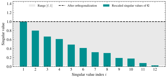
In the plot, the teal bars are one matrix’s singular values, rescaled so the largest is \(1\), and the black dashed line is where orthogonalization sends all of them. The shaded band is the interval \([\ell,1]\) that the rescaled singular values occupy, with \(\ell\) the smallest of them; the band is wide here because this matrix has condition number \(\kappa = \sigma_1/\sigma_r = 1/\ell \approx 38\), the Optimization lecture’s measure of how stretched a problem is. Collapsing that band onto the dashed line is all orthogonalization does, and it is all Muon does.
That should bother you. A nearly rank-one gradient and a perfectly flat one with the same singular vectors receive the identical update. Have we thrown away the gradient’s own weighting of which directions matter? We have, and on purpose. A budget on the worst-case stretch is already fully spent by the top direction, so holding the others back makes the step no cheaper and the loss decrease smaller. This is the complaint the Optimization lecture made about one learning rate serving a stretched bowl, answered from the other side: there we rescaled the features to round out the geometry, here we reshape the step so no direction is starved.
One thing stands between us and an optimizer: \(\mathbf{U}\) and \(\mathbf{V}\) come out of an SVD, and a training step cannot afford one.
Cheap Orthogonalization via Newton–Schulz
The case for avoiding the SVD is not asymptotic, since an SVD and a handful of same-shape matrix multiplications both cost \(O(dk\min(d,k))\); it is that matrix multiplication is the one operation accelerators run at full throughput and at the low precision training already uses, while an SVD parallelizes badly and wants high precision. So we want the polar factor expressed in matrix multiplications and nothing else.
The Newton–Schulz iteration does that. Rescale the gradient so that all of its singular values are at most \(1\), which dividing by the Frobenius norm accomplishes since \(\sigma_1\leq\|\mathbf{G}\|_F\): \[ \mathbf{X}^{(0)} = \frac{\mathbf{G}}{\|\mathbf{G}\|_F} . \] Write \(\ell>0\) for the smallest nonzero singular value of \(\mathbf{X}^{(0)}\), as in the spectrum figure, so that every singular value of \(\mathbf{X}^{(0)}\) is either \(0\) or lies in the interval \([\ell,1]\). Then repeat the cubic step \[ \mathbf{X}^{(t+1)} = \frac32\mathbf{X}^{(t)} - \frac12\,\mathbf{X}^{(t)}\big(\mathbf{X}^{(t)}\big)^\top\mathbf{X}^{(t)} , \] which is two matrix multiplications and a weighted sum, nothing else.
Why should a cubic in \(\mathbf{X}\) have anything to do with singular values at all? Because of the following fact, which we prove at the board in class.
Claim: Let \(q(x) = c_1x + c_3x^3 + c_5x^5 + \cdots\) be a polynomial with only odd powers, and define its matrix version by replacing each \(x^{2m+1}\) with \(\mathbf{X}(\mathbf{X}^\top\mathbf{X})^m\): \[ q(\mathbf{X}) = c_1\mathbf{X} + c_3\,\mathbf{X}\mathbf{X}^\top\mathbf{X} + c_5\,\mathbf{X}\mathbf{X}^\top\mathbf{X}\mathbf{X}^\top\mathbf{X} + \cdots . \] If \(\mathbf{X} = \mathbf{U}\mathbf{\Sigma}\mathbf{V}^\top\), then \(q(\mathbf{X}) = \mathbf{U}\,q(\mathbf{\Sigma})\,\mathbf{V}^\top\): the singular vectors come through untouched and \(q\) is applied to each singular value on its own.
Proof of Claim
Every term is \(\mathbf{X}(\mathbf{X}^\top\mathbf{X})^m\) for some \(m\geq0\) (the \(m=0\) term is \(\mathbf{X}\) itself), so it is enough to handle one such term. Substitute the SVD and collapse the interior with orthonormality of the singular vectors: \[ \begin{align*} \mathbf{X}^\top\mathbf{X} &= \mathbf{V}\mathbf{\Sigma}\mathbf{U}^\top\mathbf{U}\mathbf{\Sigma}\mathbf{V}^\top = \mathbf{V}\mathbf{\Sigma}^2\mathbf{V}^\top \\ (\mathbf{X}^\top\mathbf{X})^m &= \mathbf{V}\mathbf{\Sigma}^{2m}\mathbf{V}^\top \\ \mathbf{X}(\mathbf{X}^\top\mathbf{X})^m &= \mathbf{U}\mathbf{\Sigma}\mathbf{V}^\top\mathbf{V}\mathbf{\Sigma}^{2m}\mathbf{V}^\top = \mathbf{U}\mathbf{\Sigma}^{2m+1}\mathbf{V}^\top , \end{align*} \] using \(\mathbf{U}^\top\mathbf{U} = \mathbf{I}\) on the first line, then \(\mathbf{V}^\top\mathbf{V} = \mathbf{I}\) repeatedly to multiply out the \(m\)th power on the second, and once more on the third. Adding the terms back up with their coefficients, \[ q(\mathbf{X}) = \mathbf{U}\Big(\sum_m c_{2m+1}\mathbf{\Sigma}^{2m+1}\Big)\mathbf{V}^\top = \mathbf{U}\,q(\mathbf{\Sigma})\,\mathbf{V}^\top , \] and \(\mathbf{\Sigma}\) is diagonal, so \(q(\mathbf{\Sigma})\) is the diagonal matrix whose \(i\)th entry is \(q(\sigma_i)\).The Newton–Schulz step is this claim applied to one particular cubic: \[ p(x) = \frac{3x-x^3}{2} . \] The iteration on matrices is an iteration on numbers, run in parallel on every singular value at once, so we never compute \(\mathbf{U}\) or \(\mathbf{V}\) and never need to. All we need is a polynomial that sends every number in \([\ell,1]\) to \(1\), and sends \(0\) to \(0\) so that unused directions stay unused.
Fixed Points and Convergence
Let’s find where \(p\) sends a number, exactly as we will in class. The fixed points solve \(x = p(x)\): \[ x = \frac{3x-x^3}{2} \iff 2x = 3x-x^3 \iff x^3-x = 0 \iff x(x-1)(x+1) = 0 , \] so \(p\) fixes \(x=-1\), \(x=0\), and \(x=1\), and nothing else. Two of those are exactly the values we want held in place: a singular value already at \(1\) stays put, and a direction the gradient never uses stays at \(0\). The question is what happens to everything in between. Start at a small singular value \(x^{(0)}=0.1\) and iterate twice: \[ x^{(1)} = \frac{3(0.1)-(0.1)^3}{2} = \frac{0.3-0.001}{2} = 0.1495, \qquad x^{(2)} = \frac{3(0.1495)-(0.1495)^3}{2} \approx 0.2226 . \] Each step multiplied the number by about \(3/2\), which is what the cubic does while \(x^3\) is negligible next to \(3x\), since \(p(x)\approx\frac32x\) near zero. As \(x\) approaches \(1\), the cubic term cancels the excess exactly and pins the value there: small singular values climb slowly at first and only snap into place once they are close to \(1\), which is why a badly conditioned gradient needs more Newton–Schulz iterations.
Problem 18 turns that convergence into a proof. Orthogonalizing \(\mathbf{X}^{(0)}\) means driving the whole interval \([\ell,1]\) to the single point \(1\), so the only state that matters after \(t\) steps is one number: the image of \(\ell\) under \(t\) applications of \(p\). The problem shows that \(p\) is increasing on \([0,1]\), that it therefore maps \([\ell,1]\) to a strictly smaller interval \([p(\ell),1]\), and that repeating this one fixed cubic forever sends every nonzero singular value to exactly \(1\). Practical implementations do better by changing the polynomial as they go: at each step, pick the odd polynomial that lifts the current worst point \(\ell_t\) as high as a bounded-degree polynomial can. That is the Polar Express of Amsel, Persson, Musco, and Gower, the orthogonalization routine Muon implementations use in place of a fixed cubic.
The Unifying Abstraction
The last two sections applied a scalar function to a matrix’s singular values and left its singular vectors alone, the move this whole unit has been making. The Low-rank Approximation lecture’s truncated SVD is \(f(\sigma)=\sigma\) for the top \(k\) singular values and \(f(\sigma)=0\) for the rest. The pseudoinverse, from the Optimization lecture, is \(f(\sigma)=1/\sigma\) for every \(\sigma>0\) and \(f(0)=0\). Today’s orthogonalization is \(f(\sigma)=1\) for every \(\sigma>0\) and \(f(0)=0\), which is \(\mathrm{sign}\) on the nonnegative numbers. Three operations that look nothing alike are one recipe with three choices of \(f\): \[ f\Big(\sum_i \sigma_i\mathbf{u}_i\mathbf{v}_i^\top\Big) = \sum_i f(\sigma_i)\,\mathbf{u}_i\mathbf{v}_i^\top . \] The singular vectors are the geometry and always survive, while \(f\) decides what becomes of the magnitudes: truncation deletes the weak ones, the pseudoinverse inverts them, and orthogonalization forgets them entirely. What is left is to package it as an optimizer we can actually run.
Muon in Practice
Muon puts the orthogonalized step together with momentum from the Gradient Descent lecture. One step, for one weight matrix \(\mathbf{W}\):
- Compute the minibatch gradient \(\mathbf{G}^{(t)}\) and fold it into a momentum buffer, \(\mathbf{M}^{(t)} = \beta\mathbf{M}^{(t-1)} + \mathbf{G}^{(t)}\), with \(\beta\) near \(0.9\) as usual.
- Orthogonalize the momentum rather than the raw gradient: run a few Newton–Schulz steps starting from \(\mathbf{M}^{(t)}/\|\mathbf{M}^{(t)}\|_F\) to get an approximate polar factor \(\mathbf{O}^{(t)}\).
- Take the step \(\mathbf{W}^{(t+1)} = \mathbf{W}^{(t)} - \alpha\,\mathbf{O}^{(t)}\).
Five Newton–Schulz steps is the usual choice, so the added cost is about ten matrix multiplications per weight matrix per step. It is the momentum that gets orthogonalized because momentum is the direction we actually intend to move; averaging first also keeps a single noisy minibatch from deciding which directions count as used.
Two practical notes. Muon applies only to parameters that are genuinely matrices; biases and gains, which are not linear maps, are left to Adam. And since \(\|\mathbf{O}^{(t)}\|_2\approx1\) by construction, every Muon step has spectral norm about \(\alpha\) whatever the gradient’s size, so the learning rate sets the step size directly instead of only scaling it.
The conditioning payoff connects back to the Depth-enablers lecture: a deep network’s end-to-end behavior depends on a product of many weight matrices, whose conditioning degrades when individual matrices develop a few dominant singular directions. An update whose own singular values are all \(1\) moves every direction it touches by the same amount, so it does not concentrate a weight matrix’s spectrum the way a raw gradient step does.
The class demo trains the same small network on MNIST two ways, Adam against Muon, changing nothing but the optimizer. The orthogonalized step drives the training loss down considerably faster, while test accuracy moves less: optimizing faster and generalizing better turn out to be separate questions.
Looking Forward
This closes the Low-Rank Structure unit where it began, on the SVD, and answers the opening question: yes, optimization goes differently when we remember that a weight matrix is a linear map, following the polar factor of the gradient instead of the gradient.
The next unit stops asking how to train a network and starts asking what the network should be. Convolutions, attention, and the transformer are constraints imposed on the weight matrices themselves, decided before any gradient step, because some structure in the data is worth building in rather than learning from scratch.
Decide what “a small step” means before you optimize: the norm you measure steps with picks the algorithm for you.