Train a small convolutional network on handwritten digits, inspect the \(5\times5\) kernels it learned, and use class activation maps to watch where in the image it looks before it answers.
import numpy as npimport matplotlib.pyplot as pltimport scienceplotsimport torchimport torch.nn as nnfrom matplotlib.colors import LinearSegmentedColormapfrom sklearn.datasets import fetch_openmlplt.style.use(["science", "no-latex"])TEAL, CARDINAL, GRAY ="#009090", "#9c1b33", "#c9c9c9"KERNEL_CMAP = LinearSegmentedColormap.from_list("course_div", [CARDINAL, "white", TEAL])FEATURE_CMAP = LinearSegmentedColormap.from_list("course_seq", ["white", TEAL])CAM_CMAP = LinearSegmentedColormap.from_list("course_cam", [(0, 0.5, 0.5, 0.0), (0, 0.5, 0.5, 0.85)])torch.manual_seed(19)rng = np.random.default_rng(19)X, y = fetch_openml("mnist_784", version=1, return_X_y=True, as_frame=False, parser="auto")y = y.astype(int)idx = rng.choice(len(X), size=22000, replace=False)X, y = X[idx] /255.0, y[idx]n_train =20000Xtr = torch.tensor(X[:n_train].reshape(-1, 1, 28, 28), dtype=torch.float32)ytr = torch.tensor(y[:n_train], dtype=torch.long)Xte = torch.tensor(X[n_train:].reshape(-1, 1, 28, 28), dtype=torch.float32)yte = torch.tensor(y[n_train:], dtype=torch.long)class CNN(nn.Module):def__init__(self):super().__init__()self.conv1 = nn.Conv2d(1, 8, kernel_size=5, padding=2) # 8 kernels of 5x5self.conv2 = nn.Conv2d(8, 16, kernel_size=5, padding=2) # 16 kernels of 5x5x8self.head = nn.Linear(16, 10)def feature_maps(self, x): h = torch.max_pool2d(torch.relu(self.conv1(x)), 2) # 8 maps, 14x14 h = torch.max_pool2d(torch.relu(self.conv2(h)), 2) # 16 maps, 7x7return hdef forward(self, x):returnself.head(self.feature_maps(x).mean(dim=(2, 3))) # global average, then linearmodel = CNN()for name, param in model.named_parameters():print(f"{name:12s}{str(tuple(param.shape)):16s}{param.numel():>6,} parameters")print(f"{'total':29s}{sum(p.numel() for p in model.parameters()):>6,} parameters")
How good is that for the parameter budget? Train the fully connected network from the Finetuning lecture (\(784\)–\(128\)–\(10\)) on the same images, with the same optimizer, the same learning rate, and the same number of epochs.
torch.manual_seed(20)mlp = nn.Sequential(nn.Linear(784, 128), nn.ReLU(), nn.Linear(128, 10))opt = torch.optim.Adam(mlp.parameters(), lr=5e-3)Xtr_flat, Xte_flat = Xtr.reshape(-1, 784), Xte.reshape(-1, 784)for epoch inrange(20): perm = torch.randperm(len(Xtr_flat))for i inrange(0, len(Xtr_flat), 128): batch = perm[i:i +128] opt.zero_grad() lossfn(mlp(Xtr_flat[batch]), ytr[batch]).backward() opt.step()with torch.no_grad(): acc_mlp = (mlp(Xte_flat).argmax(dim=1) == yte).float().mean().item()n_cnn =sum(p.numel() for p in model.parameters())n_mlp =sum(p.numel() for p in mlp.parameters())print(f"CNN: {acc_cnn:.1%} accuracy from {n_cnn:>7,} parameters")print(f"Fully connected: {acc_mlp:.1%} accuracy from {n_mlp:>7,} parameters ({n_mlp / n_cnn:.0f}x more)")
CNN:             95.9% accuracy from   3,594 parameters
Fully connected: 96.8% accuracy from 101,770 parameters (28x more)
Essentially the same accuracy, from \(28\times\) fewer parameters. The fully connected model spends \(100{,}480\) parameters on its first layer alone, more than the whole convolutional network by a factor of nearly thirty.
The learned kernels
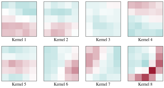
In lecture we slid the hand-picked kernel \((-1, 0, 1)\) across a signal and found an edge detector. Here are the eight \(5\times5\) kernels the first layer chose to learn (teal positive, cardinal negative).
Almost every kernel is an oriented light-to-dark transition: horizontal, vertical, or diagonal edge detectors, the two-dimensional version of the \((-1, 0, 1)\) kernel. Nobody asked for edge detectors; gradient descent rediscovered them.
One kernel at work
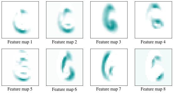
A kernel is a pattern detector, and its feature map is an image of where the pattern occurs. Slide each first-layer kernel over one test digit.
digit =0# index into the test setwith torch.no_grad(): maps = torch.relu(model.conv1(Xte[digit:digit +1]))[0].numpy() # 8 maps at full 28x28fig, axes = plt.subplots(2, 4, figsize=(7, 3.6))for k, ax inenumerate(axes.flat): ax.imshow(maps[k], cmap=FEATURE_CMAP) ax.set_xlabel(f"Feature map {k +1}") ax.set_xticks([]) ax.set_yticks([])plt.show()print(f"The digit is a {yte[digit].item()}.")
The digit is a 6.
Each map lights up on a different aspect of the same strokes (one traces the left-facing curves, another the right), and each responds to its pattern wherever it sits, because the same \(25\) weights visit every pixel.
Class activation maps
The network ends with a global average and a linear layer, so the score for class \(c\) is the spatial average of a single image, the class activation map
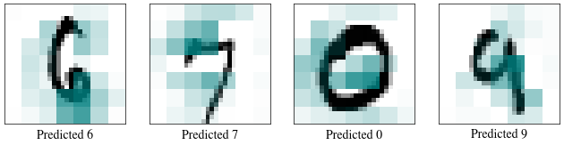
where \(\mathbf{A}_k\) is the \(k\)-th feature map of the last convolutional layer and \(w_{c,k}\) its weight in the head. Overlay each digit’s map for its predicted class.
W = model.head.weight.detach().numpy() # 10 x 16shown = [i for i inrange(len(Xte)) if preds[i] == yte[i]][:4] # first four correct predictionsfig, axes = plt.subplots(1, 4, figsize=(8, 2.4))for ax, i inzip(axes, shown):with torch.no_grad(): maps = model.feature_maps(Xte[i:i +1])[0].numpy() # 16 maps, 7x7 cam = np.maximum((W[preds[i]][:, None, None] * maps).sum(axis=0), 0) cam = np.kron(cam /max(cam.max(), 1e-9), np.ones((4, 4))) # upsample 7x7 -> 28x28 ax.imshow(Xte[i, 0].numpy(), cmap="gray_r") ax.imshow(cam, cmap=CAM_CMAP, vmin=0, vmax=1) ax.set_xlabel(f"Predicted {preds[i].item()}") ax.set_xticks([]) ax.set_yticks([])plt.show()
The heat sits on each digit’s most distinctive strokes, not uniformly over the ink.
What if we ask for a class that isn’t there?
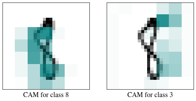
The map \(\mathrm{CAM}_c\) is defined for every class \(c\), not just the winner. Take an \(8\) from the test set and ask: which strokes would have voted for a \(3\)?
Punchline: a few thousand weights, reused at every pixel, match a hundred-thousand-parameter dense network, and because every weight has a place, we can watch the network decide where to look.