Demo: Attention Heatmaps, With and Without \(\sqrt{d_k}\)

One attention layer lets every token listen to every other token. In class we derived \(\mathrm{Var}(\langle\mathbf{q},\mathbf{k}\rangle) = d_k\) and argued that large scores saturate the softmax and kill the gradient. Here we watch both happen.

Start with the reading’s four-token example: the query of “hungry” against the keys of “the cat was hungry”, with \(d_k = 4\).

import numpy as np
import matplotlib.pyplot as plt
import scienceplots
from matplotlib.colors import LinearSegmentedColormap

plt.style.use(["science", "no-latex"])
TEAL, CARDINAL, GRAY = "#009090", "#9c1b33", "#c9c9c9"
WEIGHT_CMAP = LinearSegmentedColormap.from_list("course_seq", ["white", TEAL])

def row_softmax(S):
    e = np.exp(S - S.max(axis=-1, keepdims=True))
    return e / e.sum(axis=-1, keepdims=True)

tokens = ["the", "cat", "was", "hungry"]
q_hungry = np.array([2.0, 0, 0, 0])
keys = np.array([[-1.0, 0, 0, 0],   # the
                 [ 2.0, 0, 0, 0],   # cat
                 [ 0, 1.0, 0, 0],   # was
                 [ 0, 0, 1.0, 0]])  # hungry
dk = 4

scores = keys @ q_hungry / np.sqrt(dk)
weights = row_softmax(scores)
for t, s, a in zip(tokens, scores, weights):
    print(f"{t:>7s}: scaled score {s:5.1f} -> attention weight {a:.3f}")

    the: scaled score  -1.0 -> attention weight 0.038
    cat: scaled score   2.0 -> attention weight 0.757
    was: scaled score   0.0 -> attention weight 0.102
 hungry: scaled score   0.0 -> attention weight 0.102

“hungry” listens mostly to “cat”, the same \((0.038, 0.757, 0.102, 0.102)\) as the reading, and the layer resolved who is hungry in one step.

The full attention matrix

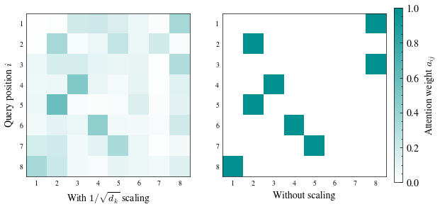
Now every query against every key. Take \(n = 8\) random tokens whose query and key entries are independent with mean zero and variance one, exactly the in-class exercise’s assumption, with a wide head, \(d_k = 256\). Compute the score matrix \(\mathbf{Q}\mathbf{K}^\top\) once with the \(1/\sqrt{d_k}\) scaling and once without, softmax each row, and draw both heatmaps. Rows are query positions \(i\) and columns are key positions \(j\).

rng = np.random.default_rng(20)
n, dk = 8, 256
Q = rng.standard_normal((n, dk))
K = rng.standard_normal((n, dk))
S = Q @ K.T

A_scaled = row_softmax(S / np.sqrt(dk))
A_unscaled = row_softmax(S)

fig, axes = plt.subplots(1, 2, figsize=(7, 3.2))
for ax, A, caption in zip(axes, [A_scaled, A_unscaled],
                          ["With $1/\\sqrt{d_k}$ scaling", "Without scaling"]):
    im = ax.imshow(A, cmap=WEIGHT_CMAP, vmin=0, vmax=1)
    ax.set_xlabel(caption)
    ax.set_xticks(range(n)); ax.set_yticks(range(n))
    ax.set_xticklabels(range(1, n + 1), fontsize=7)
    ax.set_yticklabels(range(1, n + 1), fontsize=7)
    ax.tick_params(which="both", bottom=False, left=False, top=False, right=False)
axes[0].set_ylabel("Query position $i$")
cbar = fig.colorbar(im, ax=axes, fraction=0.045, pad=0.02)
cbar.set_label("Attention weight $a_{ij}$")
plt.show()

print(f"Std of unscaled scores: {S.std():.1f}   (class prediction: sqrt({dk}) = {np.sqrt(dk):.0f})")
print(f"Std of scaled scores:   {(S / np.sqrt(dk)).std():.2f}")

Std of unscaled scores: 17.1   (class prediction: sqrt(256) = 16)
Std of scaled scores:   1.07

The exercise predicted unscaled scores of typical size \(\sqrt{256} = 16\); we measured \(17.1\). Scores that size collapse a softmax: on the right, every one of the eight rows has put nearly all of its weight on a single key, while on the left each query spreads its weight over several keys.

How saturated, exactly? Check the largest weight in each row.

print("Largest weight per row, scaled:  ", np.round(A_scaled.max(axis=1), 3))
print("Largest weight per row, unscaled:", np.round(A_unscaled.max(axis=1), 4))

Largest weight per row, scaled:   [0.351 0.351 0.312 0.493 0.579 0.437 0.328 0.346]
Largest weight per row, unscaled: [0.9998 0.9986 0.9999 1.     1.     1.     0.9998 0.9998]

The gradient dies

In class we derived the softmax Jacobian \(\partial a_j/\partial s_l = a_j(\mathbb{1}[j{=}l] - a_l)\) and argued every entry vanishes as the weights approach one-hot. Every gradient reaching \(\mathbf{W}_Q\) and \(\mathbf{W}_K\) passes through this matrix, so its size bounds how far the scores can move in one step. Compute its Frobenius norm for each row of both attention matrices.

def jacobian_norm(a):
    J = np.diag(a) - np.outer(a, a)
    return np.linalg.norm(J)

norm_scaled = np.mean([jacobian_norm(a) for a in A_scaled])
norm_unscaled = np.mean([jacobian_norm(a) for a in A_unscaled])
print(f"Mean softmax Jacobian norm, scaled:   {norm_scaled:.3f}")
print(f"Mean softmax Jacobian norm, unscaled: {norm_unscaled:.1e}")
print(f"Ratio: {norm_scaled / norm_unscaled:,.0f}x")

Mean softmax Jacobian norm, scaled:   0.368
Mean softmax Jacobian norm, unscaled: 4.8e-04
Ratio: 769x

A factor of \(769\). The unscaled head is stuck with whatever attention pattern its initialization handed it, and no gradient will move it.

What if we change the head size?

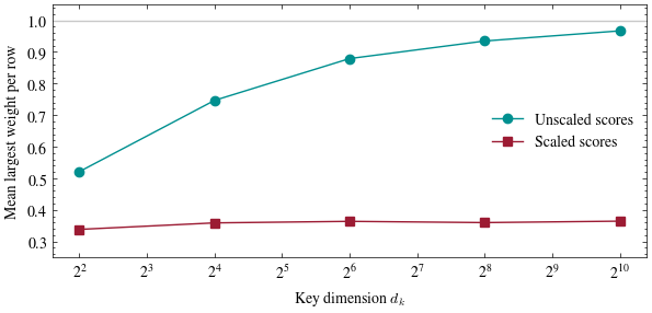
\(d_k = 256\) made the contrast stark, but is a standard head (\(d_k = 64\)) safe without scaling? Sweep the head size and track how concentrated the attention gets, averaged over many random draws.

n = 8         # change me!
dks = [4, 16, 64, 256, 1024]

rng = np.random.default_rng(21)
mean_max_unscaled, mean_max_scaled = [], []
for dk in dks:
    mx_un, mx_sc = [], []
    for _ in range(200):
        Q = rng.standard_normal((n, dk)); K = rng.standard_normal((n, dk))
        S = Q @ K.T
        mx_un.append(row_softmax(S).max(axis=1).mean())
        mx_sc.append(row_softmax(S / np.sqrt(dk)).max(axis=1).mean())
    mean_max_unscaled.append(np.mean(mx_un))
    mean_max_scaled.append(np.mean(mx_sc))

fig, ax = plt.subplots(figsize=(7, 3))
ax.plot(dks, mean_max_unscaled, "o-", color=TEAL, label="Unscaled scores")
ax.plot(dks, mean_max_scaled, "s-", color=CARDINAL, label="Scaled scores")
ax.axhline(1.0, color=GRAY, linewidth=1)
ax.set_xscale("log", base=2)
ax.set_xlabel("Key dimension $d_k$")
ax.set_ylabel("Mean largest weight per row")
ax.set_ylim(0.25, 1.05)
ax.legend(frameon=False)
plt.show()

for dk, un in zip(dks, mean_max_unscaled):
    print(f"d_k = {dk:5d}: unscaled winner takes {un:.0%} of the weight")

d_k =     4: unscaled winner takes 52% of the weight
d_k =    16: unscaled winner takes 75% of the weight
d_k =    64: unscaled winner takes 88% of the weight
d_k =   256: unscaled winner takes 93% of the weight
d_k =  1024: unscaled winner takes 97% of the weight

Without scaling, saturation grows steadily with the head size: already at the standard \(d_k = 64\), the winning key takes \(88\%\) of the weight on average, while the scaled curve doesn’t move at all. (Try a longer sequence: more keys means more competition for the softmax, so n = 100 softens both curves, but the gap survives.)

Punchline: the \(\sqrt{d_k}\) is variance control. It keeps every attention head inside the softmax’s trainable range no matter how wide the head, and without it a wide head starts saturated and never receives a usable gradient.