Positional Embeddings

Last lecture we assembled the transformer: multi-head attention, an MLP at every position, residual connections, layer normalization, and the causal mask. Not one of those pieces knows where any token sits. Our demo patched the gap with a learned table of position vectors, flagged in a comment as today’s business. The gap itself was proved two lectures ago. Self-attention is permutation-equivariant, \(\operatorname{Attention}(\mathbf{P}\mathbf{X}) = \mathbf{P}\operatorname{Attention}(\mathbf{X})\) for every permutation matrix \(\mathbf{P}\), so “dog bites man” and “man bites dog” produce the same output vectors in a different order. Today we fill the gap properly. The fix is a rotation.

How do we tell attention where its tokens are?

Absolute or Relative?

There are two ways to hand a model position, and the choice organizes the whole lecture.

The absolute approach gives each position its own vector. Keep a table \(\mathbf{p}_1, \mathbf{p}_2, \ldots \in \mathbb{R}^d\) with one entry per position, and add the right entry to each token embedding before the first block: \[ \mathbf{x}_m \;\leftarrow\; \mathbf{x}_m + \mathbf{p}_m . \] This is what our demo did, and it works: GPT-2 shipped with a learned table of exactly this form. The vectors it hands out, though, are arbitrary name tags: position \(5\)’s and position \(5000\)’s are two rows learned independently, no more connected than the embeddings of “cat” and “chandelier”.

The relative approach says that what matters is how far apart two tokens are, not where either one sits: “the token three positions back” plays the same grammatical role at position \(5\) and at position \(5000\), a subject just before its verb. Relative information also transfers where absolute tags do not. A model trained on length-\(512\) sequences updated \(\mathbf{p}_{100}\) on every training sequence and never touched \(\mathbf{p}_{1000}\), while the offset “three positions back” occurred at every position of every sequence.

So here is the design target: attention scores that depend on the query position \(m\) and the key position \(n\) only through the difference \(n - m\).

A Ladder of Frequencies

Before we hit that target, we borrow an idea from the 2017 paper that introduced the transformer. Rather than learning the table of position vectors, it computed one. Position \(m\)’s vector fills its \(d\) coordinates two at a time, with pair \(j\) holding a sine and a cosine of the same angle \(m\theta_j\): \[ \mathbf{p}_m = \big(\sin(m\theta_0),\, \cos(m\theta_0),\, \sin(m\theta_1),\, \cos(m\theta_1),\, \ldots,\, \sin(m\theta_{d/2-1}),\, \cos(m\theta_{d/2-1})\big)^\top \in \mathbb{R}^d, \] where the \(d/2\) frequencies \(\theta_j > 0\) come from a geometric ladder: \[ \theta_j = 10000^{-2j/d}, \qquad j = 0, 1, \ldots, d/2 - 1 . \] Read the ladder off at its two ends. At \(j = 0\), \(\theta_0 = 1\) and the first pair advances a full radian per position; at \(j = d/2 - 1\) the exponent is just short of \(-1\), so the last pair advances by roughly \(10^{-4}\) radians and needs thousands of tokens to move appreciably. In between, each pair is a fixed factor slower than the pair before it, which lets \(d/2\) pairs span every timescale from a single token to an entire document.

This sinusoidal embedding has one good idea and one limitation. The good idea is the ladder: nothing about it is learned, so position \(5000\) is as well defined as position \(5\) even if training never ran that far. The limitation is the operation: the embedding is still added to the content and still absolute, a fixed name tag rather than a learned one, saying nothing about \(n - m\).

We will keep the ladder and change the operation: instead of adding sines and cosines, we will use the same angles to rotate the vectors we already have.

Rotation, Not Addition

Rotary position embeddings, or RoPE, were introduced in the 2021 RoFormer paper, and they are the position mechanism inside essentially every modern open-weight language model. RoPE acts inside a single head, after the query and key projections and before the scores are formed. From here on, \(d\) is the dimension of the queries and keys within one head (the \(d_k\) of the last two lectures, typically \(64\)), and we require it to be even. To build intuition we start at \(d = 2\), where a vector is a point in the plane and a position is an angle.

Fix one frequency \(\theta > 0\) and let \(\mathbf{R}_m \in \mathbb{R}^{2\times 2}\) be the matrix that rotates the plane counterclockwise by the angle \(m\theta\): \[ \mathbf{R}_m = \begin{bmatrix} \cos(m\theta) & -\sin(m\theta) \\ \sin(m\theta) & \cos(m\theta) \end{bmatrix}. \] RoPE’s rule is simple: the query at position \(m\) becomes \(\mathbf{R}_m\mathbf{q}\), the key at position \(n\) becomes \(\mathbf{R}_n\mathbf{k}\), and the values are left alone. The further into the sequence a token sits, the further its query and key have been turned; nothing is added.

The score between positions \(m\) and \(n\) is the scaled dot product of the two rotated vectors, rewritten as a matrix product to expose the object at its center: \[ s_{mn} = \frac{\langle \mathbf{R}_m\mathbf{q}, \mathbf{R}_n\mathbf{k}\rangle}{\sqrt{d}} = \frac{(\mathbf{R}_m\mathbf{q})^\top(\mathbf{R}_n\mathbf{k})}{\sqrt{d}} = \frac{\mathbf{q}^\top\, \mathbf{R}_m^\top \mathbf{R}_n\, \mathbf{k}}{\sqrt{d}} . \] The object at the center is \(\mathbf{R}_m^\top\mathbf{R}_n\): one rotation undone, then another applied. Geometrically the two absolute angles should cancel, leaving only the gap between them, and the first in-class exercise checks that they do.

Claim: For \(2\times 2\) rotation matrices, \(\mathbf{R}_m^\top\mathbf{R}_n = \mathbf{R}_{n-m}\), and therefore the attention score depends on \(m\) and \(n\) only through the difference \(n - m\).

Proof of Claim

Write \(a = m\theta\) and \(b = n\theta\) to keep the trigonometry readable. Transposing \(\mathbf{R}_m\) flips the sign of the two off-diagonal sines, and multiplying the two matrices out entry by entry gives: \[ \begin{align*} \mathbf{R}_m^\top\mathbf{R}_n &= \begin{bmatrix} \cos a & \sin a \\ -\sin a & \cos a \end{bmatrix} \begin{bmatrix} \cos b & -\sin b \\ \sin b & \cos b \end{bmatrix} \\ &= \begin{bmatrix} \cos a\cos b + \sin a \sin b & -\cos a \sin b + \sin a \cos b \\ -\sin a\cos b + \cos a \sin b & \sin a \sin b + \cos a \cos b\end{bmatrix} \\ &= \begin{bmatrix} \cos(b-a) & -\sin(b-a) \\ \sin(b-a) & \cos(b-a)\end{bmatrix}, \end{align*} \] where the last equality is the pair of angle-subtraction formulas, \(\cos a\cos b + \sin a\sin b = \cos(b - a)\) and \(\cos a \sin b - \sin a\cos b = \sin(b - a)\). Since \(b - a = (n-m)\theta\), the four entries are exactly those of the rotation by the angle \((n-m)\theta\), which is to say \(\mathbf{R}_m^\top\mathbf{R}_n = \mathbf{R}_{n-m}\). (Geometrically this is what we expected: \(\mathbf{R}_m^\top\) rotates back by \(m\theta\) and \(\mathbf{R}_n\) rotates forward by \(n\theta\), so the net motion is forward by \((n-m)\theta\).) Substituting into the score, \[ s_{mn} = \frac{\mathbf{q}^\top \mathbf{R}_{n-m}\, \mathbf{k}}{\sqrt{d}}, \] which mentions \(m\) and \(n\) only through \(n - m\). Shift the query and the key by the same number of positions and the score does not move.

So the score is \(s_{mn} = \mathbf{q}^\top\mathbf{R}_{n-m}\mathbf{k}/\sqrt{d}\). Each token is stamped with its own absolute position, rotated the moment it is produced without knowing what it will eventually be compared against; the relative dependence appears only at the comparison, where the two rotations cancel down to the offset.

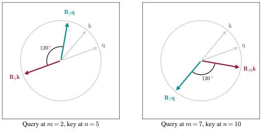
In the plot, the same content vectors \(\mathbf{q}\) and \(\mathbf{k}\) (gray) are rotated with \(\theta = \pi/6\), on the left at positions \(2\) and \(5\), on the right at \(7\) and \(10\). The rotated pairs point in completely different directions, but the angle between them is \(120^\circ\) in both panels, because the offset \(n - m = 3\) is the same. An inner product of fixed-length vectors sees that angle and nothing else, so the score is the same too, and only because rotation leaves lengths alone.

Rotations Preserve the Norm

The second in-class exercise checks a property that addition cannot offer.

Claim: Rotation preserves the norm: \(\|\mathbf{R}_m\mathbf{q}\| = \|\mathbf{q}\|\) for every position \(m\) and every \(\mathbf{q} \in \mathbb{R}^2\).

Proof of Claim

Set \(n = m\) in the identity we just proved: \[ \mathbf{R}_m^\top\mathbf{R}_m = \mathbf{R}_{m-m} = \mathbf{R}_0 = \mathbf{I}, \] since rotating by the angle \(0\) does nothing. Now expand the squared norm and use that identity in the middle: \[ \|\mathbf{R}_m\mathbf{q}\|^2 = (\mathbf{R}_m\mathbf{q})^\top(\mathbf{R}_m\mathbf{q}) = \mathbf{q}^\top\mathbf{R}_m^\top\mathbf{R}_m\mathbf{q} = \mathbf{q}^\top\mathbf{I}\mathbf{q} = \mathbf{q}^\top\mathbf{q} = \|\mathbf{q}\|^2 . \] Taking square roots of both nonnegative sides gives \(\|\mathbf{R}_m\mathbf{q}\| = \|\mathbf{q}\|\).

The proof turns on the identity at \(n = m\), \(\mathbf{R}_m^\top\mathbf{R}_m = \mathbf{R}_0 = \mathbf{I}\): rotations are orthogonal matrices, joining the permutation matrices of the Self-attention lecture and the polar factor \(\mathbf{U}\mathbf{V}^\top\) of the Muon lecture.

Why does this matter? Because a query’s length sets how loudly it speaks: scores scale linearly with \(\|\mathbf{q}\|\), and the Self-attention lecture spent a whole section and a factor of \(\sqrt{d_k}\) keeping score magnitudes near \(1\) so the softmax would not saturate and kill the gradient. Rotation changes only a query’s direction, which keys it aligns with, never its magnitude, so RoPE stamps position onto every token without disturbing that calibration.

The additive approach offers no such guarantee: the augmented vector \(\mathbf{q} + \mathbf{p}_m\) has a length that depends on \(m\), so how loudly a token speaks varies with where it sits.

Both claims concern one pair of positions; attention computes every pair at once, so let us see what shape the identity forces on the whole matrix.

The Score Matrix Is Toeplitz

Imagine one token repeated down the whole sequence, so that the score \(s_{mn}\) isolates what position alone contributes. Assemble the scores into a matrix \(\mathbf{S}\) with \([\mathbf{S}]_{m,n} = s_{mn}\). By the Claim, \([\mathbf{S}]_{m,n}\) is a function of \(n - m\) alone, so entry \((0, 3)\) equals entry \((1, 4)\) equals entry \((9, 12)\): every diagonal is constant. A matrix whose entries depend only on \(n - m\) is called Toeplitz.

We have met this structure before: Problem 19’s circular convolution matrix was constant along its diagonals too, with the extra property that they wrap around the edges, making it circulant. (Do you see why every circulant matrix is Toeplitz but not the reverse?) This is the payoff of the course’s structure arc: convolution’s weight sharing produced circulant matrices, attention’s rotary position stamps produce Toeplitz score matrices, and two architectures built for different reasons land on the same algebraic signature of “blind to absolute position, sensitive only to offsets.”

The score is also a sinusoid in the offset \(n - m\), so two offsets a full turn apart score almost identically, a repetition the rest of the lecture fixes. The class demo plots \(\mathbf{S}\) directly and confirms it: constant diagonals, to floating-point precision.

A Clock with Many Hands

One plane is not enough. A real head has \(d = 64\) dimensions, and a single angle can only say so much. RoPE’s full recipe splits the query \(\mathbf{q} \in \mathbb{R}^d\) into \(d/2\) two-dimensional slices and rotates slice \(j\) by the angle \(m\theta_j\), using the sinusoidal ladder from before, now driving rotations rather than name tags. Stacking the \(d/2\) little rotations along the diagonal gives one block-diagonal matrix: \[ \mathbf{\Theta}_m = \begin{bmatrix} \mathbf{R}_m^{(\theta_0)} & & \\ & \ddots & \\ & & \mathbf{R}_m^{(\theta_{d/2-1})}\end{bmatrix} \in \mathbb{R}^{d\times d}, \] where \(\mathbf{R}_m^{(\theta_j)}\) is the \(2\times2\) rotation by \(m\theta_j\). Block-diagonal matrices multiply block by block, so everything we proved in the plane survives intact: \[ \mathbf{\Theta}_m^\top\mathbf{\Theta}_n = \mathbf{\Theta}_{n-m}, \qquad \mathbf{\Theta}_m^\top\mathbf{\Theta}_m = \mathbf{I}, \qquad \|\mathbf{\Theta}_m\mathbf{q}\| = \|\mathbf{q}\| . \] Each block of the first product is the Claim with \(\theta_j\) in place of \(\theta\), and the other two identities follow exactly as before. So the scores of a repeated token still depend only on \(n - m\), and the score matrix is still Toeplitz.

The picture to carry away is a clock with \(d/2\) hands, hand \(j\) advancing by \(\theta_j\) radians per position.

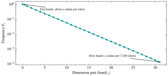
In the plot, the ladder for a \(d = 64\) head descends geometrically across its \(32\) hands, from \(\theta_0 = 1\) down to \(\theta_{31} \approx 1.3\times 10^{-4}\). The fast end turns about \(57^\circ\) per token; the slow end needs about \(7{,}500\) tokens to turn one radian.

Why does RoPE need the whole ladder instead of one well-chosen frequency? After \(2\pi \approx 6.28\) positions a single fast hand has swept a full circle, so two positions six apart land at nearly the same angle and the score cannot tell them apart. A clock with only a minute hand reads \(12{:}30\) and \(1{:}30\) identically.

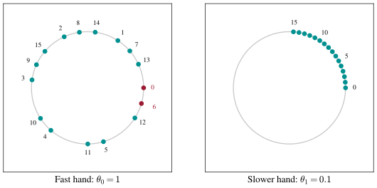
In the plot, sixteen positions are placed on two of the hands. The fast hand (\(\theta_0 = 1\)) laps the circle twice, and positions \(0\) and \(6\) (cardinal) land closer together than any two consecutive positions do. The slower hand (\(\theta_1 = 0.1\)) fans the same sixteen positions out in unambiguous order, but into a narrow wedge. Fast hands separate neighbors; slow hands separate chapters; the ladder keeps both.

Problem 22 makes this precise. It derives each hand’s period, quantifies how badly a single fast hand aliases, and shows that across a context of tens of thousands of tokens the slowest hand still assigns distinct positions distinct angles. It closes with the fact that advancing the entire clock by \(k\) positions is multiplication by one fixed matrix \(\mathbf{\Theta}_k\), independent of where in the sequence you start, which is the algebraic form of “shift by \(k\) means the same thing everywhere.”

Looking Forward

This lecture closes the Architectures unit. Convolution bet that only local interactions matter, and bought translation equivariance with weight sharing. Attention refused the bet and connected everything to everything, at the cost of knowing where nothing was. The transformer block assembled attention into the machine behind modern language models, and today a ladder of rotations gave that machine a sense of place without disturbing a single norm. The structure arc’s portable lesson: when you want a model to treat a quantity as relative, do not encode the absolute value and hope the model learns to subtract it; build the operation so that the absolute parts cancel on their own. Next lecture the final unit takes away the luxury every model so far has enjoyed, a label for every input: reinforcement learning.