Every model we trained this semester was handed the right answer for every input. Today’s agent gets a pole balanced on a cart and a single instruction: don’t drop it. The state \(s_t \in \mathbb{R}^4\) holds the cart’s position and velocity and the pole’s angle and angular velocity; the actions are push left or push right; the reward is \(+1\) for every step the pole stays up; the episode ends when the pole tips past about \(12°\), the cart leaves the track, or \(500\) steps elapse. Nobody ever says which push was correct.
import gymnasium as gymimport numpy as npimport matplotlib.pyplot as pltimport scienceplotsplt.style.use(["science", "no-latex"])TEAL, CARDINAL, GRAY ="#009090", "#9c1b33", "#c9c9c9"env = gym.make("CartPole-v1")print("State space: ", env.observation_space)print("Action space:", env.action_space)state, _ = env.reset(seed=145)print("One starting state:", state)
The loop from the reading, as code: observe the state, pick an action, receive a reward and the next state, repeat until the episode ends. The episode’s list of rewards is everything the environment ever says.
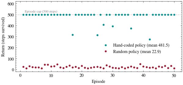
The simplest possible policy ignores the state entirely: \(\pi(a|s) = \frac12\) for both actions. The agent generates its own data, so let’s generate some: \(50\) episodes. The undiscounted return of an episode is just its length, the number of steps the pole survived.
rng = np.random.default_rng(23)def random_policy(state):returnint(rng.integers(2))random_episodes = [run_episode(env, random_policy, seed) for seed inrange(50)]random_returns = np.array([sum(ep) for ep in random_episodes])print(f"Random policy over 50 episodes: mean return {random_returns.mean():.1f}, "f"min {random_returns.min():.0f}, max {random_returns.max():.0f}")
Random policy over 50 episodes: mean return 22.9, min 10, max 51
About a second of simulated time before the pole hits the ground.
A hand-coded policy
Now a policy that actually reads the state, in one deterministic line: push in the direction the pole is leaning and falling, using the angle and angular velocity (the state’s last two coordinates, indices 2 and 3 in the code).
def lean_policy(state):return1if state[2] + state[3] >0else0lean_episodes = [run_episode(env, lean_policy, seed) for seed inrange(100, 150)]lean_returns = np.array([sum(ep) for ep in lean_episodes])print(f"Hand-coded policy over 50 episodes: mean return {lean_returns.mean():.1f}, "f"min {lean_returns.min():.0f}, max {lean_returns.max():.0f}")print(f"Episodes hitting the 500-step cap: {(lean_returns ==500).sum()} of 50")print(f"Improvement over random: {lean_returns.mean() / random_returns.mean():.1f}x")
Hand-coded policy over 50 episodes: mean return 481.5, min 275, max 500
Episodes hitting the 500-step cap: 44 of 50
Improvement over random: 21.0x
A factor of \(21\) from a single if statement. Plot every episode’s return for both policies; this is the reading’s headline figure.
The in-class exercise computed the effective horizon \(1/(1-\gamma)\): \(10\) steps at \(\gamma = 0.9\), \(100\) at \(\gamma = 0.99\). And since every CartPole reward is \(1\), those numbers are also ceilings: an episode that lasts forever earns a discounted return of exactly \(\sum_k \gamma^k = 1/(1-\gamma)\). Watch two real episodes run into them, one short random episode and one full-length balanced episode.
def discounted_return(rewards, gamma):returnsum(gamma**k * r for k, r inenumerate(rewards))short_ep, long_ep = random_episodes[0], lean_episodes[0]print(f"Random episode: {len(short_ep)} steps. Balanced episode: {len(long_ep)} steps.\n")print(f"{'':>14}{'random':>10}{'balanced':>10}{'ceiling 1/(1-gamma)':>22}")print(f"{'undiscounted':>14}{sum(short_ep):>10.2f}{sum(long_ep):>10.2f}{'(none)':>22}")for gamma in [0.9, 0.99]:print(f"{'gamma = '+str(gamma):>14}{discounted_return(short_ep, gamma):>10.2f} "f"{discounted_return(long_ep, gamma):>10.2f}{1/ (1- gamma):>22.0f}")
At \(\gamma = 0.9\), surviving \(500\) steps scores \(10.00\) and surviving \(25\) steps scores \(9.28\). Twenty times the survival buys nearly identical returns, because both episodes outlast a myopic agent’s ten-step horizon. At \(\gamma = 0.99\) the two episodes finally separate: \(22.22\) versus \(99.34\). The knob \(\gamma\) decides which behaviors the agent can even tell apart.
What if? (change me!)
Two things beg to be changed. Try GAMMA = 0.5 (an effective horizon of two steps: can any policy look good?), and try the alternative heuristic that pushes on the angle alone, ignoring the angular velocity.
GAMMA =0.5# change me: 0.5, 0.9, 0.99, 0.999USE_ANGLE_ONLY =True# change me: ignore the angular velocity?def angle_only_policy(state):return1if state[2] >0else0policy = angle_only_policy if USE_ANGLE_ONLY else lean_policywhatif_episodes = [run_episode(env, policy, seed) for seed inrange(100, 150)]whatif_returns = np.array([sum(ep) for ep in whatif_episodes])print(f"Mean return over 50 episodes: {whatif_returns.mean():.1f} "f"(hand-coded was {lean_returns.mean():.1f}, random was {random_returns.mean():.1f})")print(f"Mean discounted return at gamma = {GAMMA}: "f"{np.mean([discounted_return(ep, GAMMA) for ep in whatif_episodes]):.2f} "f"(ceiling {1/ (1- GAMMA):.0f})")
Mean return over 50 episodes: 42.1 (hand-coded was 481.5, random was 22.9)
Mean discounted return at gamma = 0.5: 2.00 (ceiling 2)
The angle-only rule reads the state and still only doubles the random policy (\(42.1\) vs. \(22.9\)): it pushes back only after the pole is already tilted, so the cart overcorrects and oscillates out of bounds. Feedback on where the pole is going (the angular velocity) is worth far more than feedback on where it is. Nothing in today’s lecture could have told us that without trying it, which is the exploration problem in miniature.
Punchline: with no dataset and no labels, the agent wrote its own data by acting, one hand-coded line multiplied its return by \(21\), and \(\gamma\) set how far into the future it could see. Next lecture, gradients replace the hand.