Reinforcement Learning
Last lecture completed the machine behind modern language models. Every model we trained this semester, from linear regression to last week’s transformer, enjoyed one luxury we never questioned: an answer key. A dataset came stapled to the correct outputs, and even language modeling manufactured labels for free, because the next token is the answer. Today, in the first lecture of the course’s final unit, we take the answer key away. Over three lectures we pose the new problem, learn a policy by gradient ascent, and cut that gradient’s variance with the control-variate coefficient from Problem 2: the estimator thread that opened the semester is the engine of the whole unit. This is also where the machine we just built ends up: the final training stage of a modern chatbot fine-tunes that same transformer with reinforcement learning from human feedback.
No Labels, No Dataset
Since the Linear Models unit, our recipe has been empirical risk minimization: collect a dataset of pairs \((\mathbf{x}^{(i)}, y^{(i)})\), pick a function class, and minimize a loss that scores each prediction against its label. Reinforcement learning breaks that recipe in three distinct ways.
No labels. A reward is a score, not an answer. When a chess program loses, the environment says “that was worth \(-1\),” not which of the forty moves was the mistake, let alone what the right move was. Compare the cross-entropy loss, which hands the model the exact correct token and the exact direction to nudge every probability.
Delayed reward. The consequences of an action arrive later, sometimes much later: the fatal wobble happens at step \(30\) and the pole hits the ground at step \(50\). Deciding which past actions deserve credit for a reward is called the credit assignment problem, and no previous unit had anything like it, because every training example scored itself instantly.
The agent generates its own data. An agent’s data is its own experience: the states it sees are the states its current behavior steers it into. A chess program that never castles collects no data about castling, so the quality of what it learns is limited by the adventurousness of how it acts, a tension we return to at the end of the lecture.
All three follow from a single substitution: the dataset has been replaced by an interaction, so we should say exactly what that interaction is.
The Agent–Environment Loop
At each time step \(t = 0, 1, 2, \ldots\), the agent observes the current state \(s_t \in \mathcal{S}\) of the environment and chooses an action \(a_t \in \mathcal{A}\), where \(\mathcal{S}\) is the set of states and \(\mathcal{A}\) the set of actions. The environment responds with a scalar reward \(r_t \in \mathbb{R}\) and the next state \(s_{t+1}\), and the loop repeats.
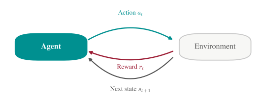
In the diagram, the top arrow is the agent’s one output, an action, and the bottom two arrows are everything the environment says back: a number and a new state. Nothing in that thin channel ever tells the agent what it should have done.
Our running example, in class and in the demo, is CartPole: a pole balances on a cart, and the agent keeps it from falling by nudging the cart. The state \(s_t \in \mathbb{R}^4\) holds the cart’s position and velocity and the pole’s angle and angular velocity; the actions are \(\mathcal{A} = \{\text{push left}, \text{push right}\}\); the reward is \(r_t = 1\) for every step the pole stays up. An episode is one run of the loop from a fresh start until the pole falls or a step limit is reached; the demo gives CartPole’s exact numbers. Doing nothing is not an option: the pole is unstable, so the agent survives only by actively steering. Steering according to what rule, though? That rule is the object we spend the rest of the unit trying to learn.
Policies
The agent’s behavior is its policy \(\pi\): for each state \(s\), a probability distribution \(\pi(a | s)\) over the actions, from which the agent samples \(a_t \sim \pi(\cdot | s_t)\). A policy is generally stochastic, meaning it rolls dice; a deterministic rule puts all the probability on one action.
Two CartPole policies will carry today’s demo. The random policy ignores the state entirely: \(\pi(a|s) = \frac12\) for both actions. The hand-coded policy is one deterministic line: push right when the pole’s angle plus its angular velocity is positive, and left otherwise. In words, push in the direction the pole is leaning and falling, read off the state’s last two coordinates. Why allow randomness at all, when the hand-coded rule looks so sensible? Two reasons: a stochastic policy keeps trying actions it currently thinks are worse (the exploration we will need shortly), and next lecture the randomness is precisely what lets us differentiate the expected reward with respect to the policy’s parameters.
Trajectories, Return, and the Discount Factor
Running a policy produces a trajectory, the alternating sequence of states, actions, and rewards the loop generates: \[ \tau = (s_0, a_0, r_0, s_1, a_1, r_1, s_2, \ldots). \] The trajectory is the agent’s version of a training example, and we score it from time \(t\) onward by its return, which discounts each future reward by how long we wait on it: \[ G_t = r_t + \gamma r_{t+1} + \gamma^2 r_{t+2} + \cdots = \sum_{k=0}^{\infty} \gamma^k r_{t+k}, \] where the discount factor \(\gamma \in [0, 1)\) shrinks the weight on each additional step of delay. (After an episode ends, the later rewards are zero.) Discounting is an interest rate on reward: just as a dollar today is worth more than a dollar next year, a unit of reward now is worth \(1/\gamma\) units of reward one step from now. Problem 23 opens with exactly this exchange rate. Discounting also keeps the infinite sum finite (the problem set makes this precise).
The definition hides a one-step recursion. Split off the \(k = 0\) term and factor \(\gamma\) out of everything that remains: \[ G_t = r_t + \gamma\left(r_{t+1} + \gamma r_{t+2} + \cdots\right) = r_t + \gamma G_{t+1}. \] In words, today’s return is today’s reward plus \(\gamma\) times tomorrow’s return. On Problem 23, taking the expectation of this identity (linearity of expectation, from lecture one) produces the Bellman consistency equation, the workhorse identity of the field.
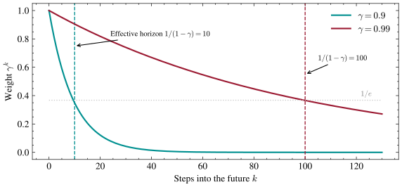
In the plot, the weight \(\gamma^k\) on a reward \(k\) steps ahead decays geometrically, and the dashed lines mark the effective horizon \(1/(1-\gamma)\), where each curve crosses the gray \(1/e\) line: at \(\gamma = 0.99\) a reward a hundred steps out still carries over a third of its face value. Both are worth a hand computation before we trust them; they are the lecture’s two in-class exercises.
Worked Example: A Four-Step Episode
The first in-class exercise makes the return and its recursion concrete. Take a four-step episode with these rewards: \[ r_0 = 1, \quad r_1 = 0, \quad r_2 = 2, \quad r_3 = 4, \] and \(\gamma = 0.9\). Summing the weighted terms gives \(G_0 = 5.536\), and the recursion \(G_t = r_t + \gamma G_{t+1}\) checks out at every step.
Solution to the class exercise
The return from the start follows by summing the four weighted terms directly: \[ G_0 = r_0 + \gamma r_1 + \gamma^2 r_2 + \gamma^3 r_3 = 1 + (0.9)(0) + (0.81)(2) + (0.729)(4) = 1 + 0 + 1.62 + 2.916 = 5.536. \] The same summation started at each later step gives the remaining three returns: \[ G_1 = 0 + (0.9)(2) + (0.81)(4) = 5.04, \qquad G_2 = 2 + (0.9)(4) = 5.6, \qquad G_3 = 4. \] Now verify the recursion \(G_t = r_t + \gamma G_{t+1}\) at \(t = 0\) by computing both sides. The left side is \(G_0 = 5.536\) from the direct sum, and the right side is: \[ r_0 + \gamma G_1 = 1 + (0.9)(5.04) = 1 + 4.536 = 5.536. \] The two sides agree, and the same check goes through at \(t = 1\) and \(t = 2\).Sweeping back to front, the recursion computes each return with one multiplication and one addition; every reinforcement learning implementation computes returns this way, including next lecture’s.
Worked Example: The Effective Horizon
The second exercise asks how far into the future a discounted agent effectively sees. The answer is the effective horizon \(1/(1-\gamma)\), roughly the number of future steps that still matter non-negligibly: \(10\) steps at \(\gamma = 0.9\) and \(100\) at \(\gamma = 0.99\).
Solution to the class exercise
Sum the weights over all future steps with the geometric series formula: \[ \sum_{k=0}^{\infty} \gamma^k = \frac{1}{1 - \gamma}. \] Two facts justify the name effective horizon: the first \(1/(1-\gamma)\) steps contribute the bulk of the total weight, and by step \(1/(1-\gamma)\) the weight has decayed by a factor of \(e \approx 2.718\). (That second fact is the compound-interest limit: \(\gamma^{1/(1-\gamma)} = (1 - (1-\gamma))^{1/(1-\gamma)} \approx e^{-1}\) when \(\gamma\) is close to \(1\).) Comparing the two values in the plot above: \[ \gamma = 0.9: \quad \frac{1}{1 - 0.9} = 10, \qquad\qquad \gamma = 0.99: \quad \frac{1}{1 - 0.99} = 100. \]Moving \(\gamma\) from \(0.9\) to \(0.99\) looks like a small nudge, and it is a tenfold extension of the agent’s sight. The two numbers have a second reading: when every reward equals \(1\), as in CartPole, an episode that never ends earns exactly \(\sum_k \gamma^k = 1/(1-\gamma)\), so \(10\) and \(100\) are ceilings on the discounted return. The demo watches two very different episodes run into them.
The Markov Decision Process
We have been informal about what the environment is; the standard formalization is the Markov decision process (MDP). An MDP consists of the state space \(\mathcal{S}\), the action space \(\mathcal{A}\), a transition distribution \(\Pr(s_{t+1} | s_t, a_t)\) over next states, the reward \(r_t\) produced alongside each transition, and the discount factor \(\gamma\). The load-bearing assumption sits in the transition distribution’s arguments, the Markov property: the next state depends only on the current state and action, not on the rest of the history. That is what the word “state” means here, a summary of the past sufficient to predict the future. CartPole’s four numbers qualify: Newtonian mechanics computes the next configuration from them alone; how the pole got to its current lean is irrelevant. (When the observation is not a sufficient summary, a single video-game frame showing positions but not velocities, the theory gets harder; we assume fully observed states.)
Maximizing Expected Return
A trajectory is random twice over: the policy rolls dice to pick actions, and the environment rolls dice to pick next states. So the return \(G_0\) is a random variable, and the objective is its expectation: \[ \max_{\pi} \; J(\pi) = \mathbb{E}_{\tau \sim \pi}\left[G_0\right] = \mathbb{E}_{\tau \sim \pi}\left[\sum_{t=0}^{\infty} \gamma^t r_t\right], \] where \(\tau \sim \pi\) denotes a trajectory generated by running the policy \(\pi\) in the MDP. We cannot compute this expectation exactly, since summing over all trajectories is hopeless, but we can sample from it by running episodes, precisely the situation the Monte Carlo estimator of lecture two was built for; next lecture we estimate both \(J(\pi)\) and its gradient by averaging sampled trajectories. Sampling from \(\pi\) carries a catch that no fixed dataset ever had: the policy we are evaluating is also the policy that decides what we get to see.
Exploration vs. Exploitation
One genuinely new tension remains, and it exists because the agent generates its own data. At any moment the agent has a best guess about which actions pay; should it exploit that guess, or explore an action that currently looks worse? Do you see the trap? An agent can be permanently wrong while feeling perfectly successful, because the experience that would correct it is exactly the experience its policy refuses to gather.
Our hand-coded CartPole policy makes the trap concrete: an agent that exploits it keeps collecting the same trajectories forever, never finding out whether some other rule does better, because every episode it runs describes only the states this one rule visits. Stochastic policies are the simplest hedge: keep \(\pi(a|s) > 0\) for every action, so everything gets tried occasionally (exploring optimally is a theory of its own, multi-armed bandits; the policies of the next two lectures explore by staying random).
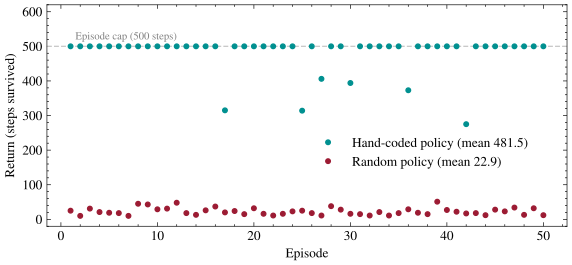
In the plot, every episode’s return under each policy is a dot: the random policy’s cloud hugs the bottom, while the hand-coded policy rides the episode cap with a handful of unlucky starts falling short. The demo runs both policies for fifty episodes, re-scores two of them at the discounts from the worked example above, and springs the trap with a third policy, walk through the numbers there.
Looking Forward
What we conspicuously did not do today is learn: our best policy was hand-coded, and hand-coding does not scale past a pole on a cart. Next lecture we make the policy a neural network \(\pi_{\boldsymbol\theta}\) and ascend the gradient \(\nabla_{\boldsymbol\theta} \mathbb{E}[G_0]\); differentiating through an expectation over the policy’s own randomness is the job of the log-derivative trick. Before then, Problem 23 turns $100-today-or-$100-next-year into mathematics: the recursion becomes the Bellman consistency equation for the value function \(V^\pi\), and \(\gamma\) turns out to be a bias–variance knob on a Monte Carlo estimator. Keep an eye on that value function: it is exactly the baseline the final lecture subtracts to cut the variance of policy gradients. The sentence to carry out of today: when the only access you have to an objective is samples you generate yourself, how you act decides what you are able to learn.