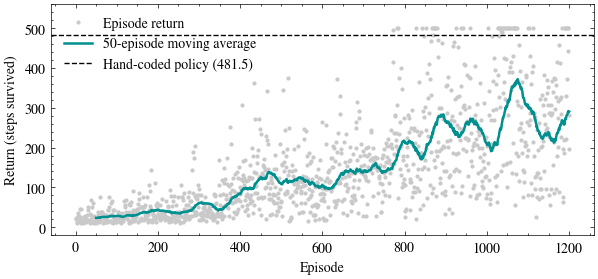
Last lecture’s best policy was a hand-coded if statement scoring \(481.5\); the random policy scored \(22.9\). Today nobody hand-codes anything: a small neural network starts as the random policy and learns to balance the pole with REINFORCE. The policy is the classifier architecture we’ve built all semester (state in, two logits out, softmax over the actions), with \(226\) parameters.
import gymnasium as gymimport numpy as npimport matplotlib.pyplot as pltimport scienceplotsimport torchimport torch.nn as nnplt.style.use(["science", "no-latex"])TEAL, CARDINAL, GRAY ="#009090", "#9c1b33", "#c9c9c9"env = gym.make("CartPole-v1")torch.manual_seed(5)policy = nn.Sequential(nn.Linear(4, 32), nn.ReLU(), nn.Linear(32, 2))print("Parameters:", sum(p.numel() for p in policy.parameters()))
Parameters: 226
The REINFORCE loop
One update per episode, exactly the four lines from the reading: run an episode sampling \(a_t \sim \pi_{\boldsymbol\theta}(\cdot|s_t)\) and recording each \(\log \pi_{\boldsymbol\theta}(a_t|s_t)\), compute the return \(G(\tau)\) back to front with last lecture’s recursion \(G_t = r_t + \gamma G_{t+1}\), then ascend \(G(\tau) \sum_t \nabla_{\boldsymbol\theta} \log \pi_{\boldsymbol\theta}(a_t|s_t)\). We implement the ascent step as a descent step on the loss \(-G(\tau)\sum_t \log \pi_{\boldsymbol\theta}(a_t|s_t)\), so loss.backward() does the work. One episode per update is \(N = 1\), the noisiest legal Monte Carlo estimate, and unbiased all the same.
episode  200: last-100 mean return 37.5
episode  400: last-100 mean return 63.9
episode  600: last-100 mean return 114.6
episode  800: last-100 mean return 177.3
episode 1000: last-100 mean return 236.3
episode 1200: last-100 mean return 261.9
Did it learn?
Compare the network before it knew anything to the network after \(1200\) episodes of its own experience.
returns = np.array(returns)first, last = returns[:50].mean(), returns[-50:].mean()print(f"First 50 episodes: mean return {first:.1f} (random policy last lecture: 22.9)")print(f"Last 50 episodes: mean return {last:.1f} (hand-coded policy: 481.5)")print(f"Improvement: {last / first:.1f}x, with {(returns ==500).sum()} episodes hitting the 500-step cap")
First 50 episodes: mean return 23.7   (random policy last lecture: 22.9)
Last 50 episodes:  mean return 290.5   (hand-coded policy: 481.5)
Improvement: 12.3x, with 45 episodes hitting the 500-step cap
A twelvefold improvement, and nobody ever said which push was correct. Plot every episode and notice how jagged it is: single-episode gradient estimates are unbiased but very noisy, so the curve lurches through progress, collapse, and recovery.
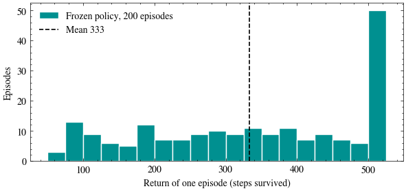
Every update scaled the whole \(226\)-coordinate gradient by one scalar: the episode’s return. Freeze the trained policy (not one weight changes from here on) and measure how much that scalar swings across \(200\) episodes.
eval_returns = []with torch.no_grad():for i inrange(200): state, _ = env.reset(seed=2000+ i) done, total =False, 0.0whilenot done: logits = policy(torch.tensor(state, dtype=torch.float32)) action = torch.distributions.Categorical(logits=logits).sample() state, reward, terminated, truncated, _ = env.step(int(action)) total += reward done = terminated or truncated eval_returns.append(total)eval_returns = np.array(eval_returns)print(f"Frozen policy over 200 episodes: mean {eval_returns.mean():.1f}, "f"std {eval_returns.std():.1f}, min {eval_returns.min():.0f}, max {eval_returns.max():.0f}")fig, ax = plt.subplots(figsize=(7, 3))ax.hist(eval_returns, bins=np.arange(50, 526, 25), color=TEAL, edgecolor="white", label="Frozen policy, 200 episodes")ax.axvline(eval_returns.mean(), color="black", linewidth=1.2, linestyle="--", label=f"Mean {eval_returns.mean():.0f}")ax.set_xlabel("Return of one episode (steps survived)")ax.set_ylabel("Episodes")ax.legend(frameon=False, loc="upper left")plt.show()
Frozen policy over 200 episodes: mean 333.0, std 144.5, min 70, max 500
The same fixed policy survives anywhere from \(70\) to \(500\) steps, a factor of seven, with standard deviation \(144.5\). Discounting compresses that spread into the multiplier the gradient actually sees: at \(\gamma = 0.99\) those two episodes score \(G(\tau) = 50.5\) and \(99.3\), still a factor of two. Either way, REINFORCE scales its entire gradient by whichever number it happens to draw, which is why the learning rate had to be timid.
What if? (change me!)
Try LR_WHATIF = 3e-2 (ten times larger: do bigger steps learn faster?) and 3e-4 (ten times smaller).
LR_WHATIF =3e-2# change me: 3e-4, 3e-3, 3e-2torch.manual_seed(5)policy_w = nn.Sequential(nn.Linear(4, 32), nn.ReLU(), nn.Linear(32, 2))optimizer_w = torch.optim.Adam(policy_w.parameters(), lr=LR_WHATIF)returns_w = []for episode inrange(N_EPISODES): state, _ = env.reset(seed=episode) log_probs, rewards, done = [], [], Falsewhilenot done: logits = policy_w(torch.tensor(state, dtype=torch.float32)) dist = torch.distributions.Categorical(logits=logits) action = dist.sample() log_probs.append(dist.log_prob(action)) state, reward, terminated, truncated, _ = env.step(int(action)) rewards.append(reward) done = terminated or truncated G =0.0for r inreversed(rewards): G = r + GAMMA * G loss =-G * torch.stack(log_probs).sum() optimizer_w.zero_grad() loss.backward() optimizer_w.step() returns_w.append(sum(rewards))returns_w = np.array(returns_w)print(f"lr = {LR_WHATIF}: first 50 mean {returns_w[:50].mean():.1f}, "f"last 50 mean {returns_w[-50:].mean():.1f} (lr = 3e-3 reached {last:.1f})")
lr = 0.03: first 50 mean 12.3, last 50 mean 9.3 (lr = 3e-3 reached 290.5)
At ten times the learning rate the policy collapses to a return of \(9.3\), worse than random, because a single noisy update is now large enough to destroy the network; at a tenth of the learning rate, \(1200\) episodes barely move it. The variance of the estimator is what pins the learning rate, and (a peek at next lecture) subtracting a baseline from \(G(\tau)\) before it multiplies the gradient is what will loosen that pin.
Punchline: the network wrote its own labels, up-weighting the log-probabilities of its own actions in proportion to the return that followed, and a twelvefold improvement fell out of gradient ascent; the jagged curve is the price of estimating a gradient from one noisy episode, and next lecture’s baseline brings it down.