Baseline and Advantage
Last lecture REINFORCE learned CartPole from scratch, climbing from a return of \(23.7\) to \(290.5\), but its training curve lurched through progress, collapse, and recovery. We traced the jaggedness to its source: one noisy scalar, the return \(G(\tau)\), multiplies the entire \(226\)-coordinate gradient. CartPole’s returns are also all positive, so no update ever pushes probability away from an action: what distinguishes a good episode from a bad one is a small difference on top of a large number they share. Problem 24 put the pathology under a microscope: shift both of a bandit’s rewards by the same constant \(c\), and the true gradient does not move while the estimator’s variance grows like \(c^2\). An estimator whose quality depends on where the reward scale puts zero needs fixing, and the fix has been in our toolbox since week two: the last lecture of the course uses the oldest tool we own.
The Baseline
Recall last lecture’s estimator, written for a single episode: \[ \widehat{\nabla J} = G(\tau) \sum_{t \geq 0} \nabla_{\boldsymbol\theta} \log \pi_{\boldsymbol\theta}(a_t | s_t), \] an unbiased Monte Carlo estimate of \(\nabla_{\boldsymbol\theta} J(\boldsymbol\theta)\), the gradient of the expected return \(J(\boldsymbol\theta) = \mathbb{E}_{\tau \sim \pi_{\boldsymbol\theta}}[G(\tau)]\). Instead of weighting each episode’s score by its raw return, we propose to weight it by the return measured against a reference level \(b \in \mathbb{R}\), a scalar called a baseline: \[ \widehat{\nabla J}^{\,b} = \big(G(\tau) - b\big) \sum_{t \geq 0} \nabla_{\boldsymbol\theta} \log \pi_{\boldsymbol\theta}(a_t | s_t). \] Read it as grading on a curve: an episode that beats par pushes probability toward its actions, an episode below par pushes away, and “how good is this number, really?” no longer depends on where zero sits. But last lecture’s log-derivative trick derived the raw return as the weight that makes the estimator unbiased. Are we not about to bend the gradient?
Claim: For any baseline \(b\) that does not depend on the actions taken, \(\mathbb{E}_{\tau \sim \pi_{\boldsymbol\theta}}\left[b \, \nabla_{\boldsymbol\theta} \log p_{\boldsymbol\theta}(\tau)\right] = \mathbf{0}\), and therefore \(\mathbb{E}[\widehat{\nabla J}^{\,b}] = \nabla_{\boldsymbol\theta} J(\boldsymbol\theta)\) for every such \(b\).
Proof of Claim
The engine is a fact about the score, the gradient of the log-probability: it has mean zero under its own distribution. For any distribution \(p_{\boldsymbol\theta}\) over outcomes \(x\), the expected score vanishes: \[ \mathbb{E}_{x \sim p_{\boldsymbol\theta}}\left[\nabla_{\boldsymbol\theta} \log p_{\boldsymbol\theta}(x)\right] = \sum_x p_{\boldsymbol\theta}(x) \, \frac{\nabla_{\boldsymbol\theta} \, p_{\boldsymbol\theta}(x)}{p_{\boldsymbol\theta}(x)} = \nabla_{\boldsymbol\theta} \sum_x p_{\boldsymbol\theta}(x) = \nabla_{\boldsymbol\theta} \, 1 = \mathbf{0}, \] where we applied the log-derivative identity from last lecture, cancelled the \(p_{\boldsymbol\theta}(x)\)’s, moved the gradient outside the sum (linearity again), and used that probabilities sum to one no matter what \(\boldsymbol\theta\) is, so the gradient of that sum is the gradient of a constant. Taking \(x = \tau\), a constant baseline contributes \(b \cdot \mathbb{E}[\nabla_{\boldsymbol\theta} \log p_{\boldsymbol\theta}(\tau)] = \mathbf{0}\), and by linearity of expectation the baselined estimator has the same mean as the raw one. The same argument covers a baseline \(b(s_t)\) that varies with the state: conditioned on \(s_t\), the inner expectation \(\mathbb{E}_{a_t \sim \pi_{\boldsymbol\theta}(\cdot|s_t)}[\nabla_{\boldsymbol\theta} \log \pi_{\boldsymbol\theta}(a_t|s_t)]\) is zero at every state by the identity above, so \(\mathbb{E}[b(s_t)\, \nabla_{\boldsymbol\theta} \log \pi_{\boldsymbol\theta}(a_t|s_t)] = \mathbf{0}\) term by term.A policy cannot raise the probability of every action at once, so a baseline’s push, spread across the actions in proportion to how often the policy takes them, cancels itself exactly. Do you see where the argument breaks if \(b\) depends on the action the agent actually took?
Every action-independent \(b\) is legal, so the whole question is which one to pick. We have chosen exactly this kind of constant once before.
A Control Variate
In the Monte Carlo lecture’s control variate section, we shrank an estimator’s variance by subtracting \(c\,(g(X) - \mathbb{E}[g])\). A surrogate quantity \(g\), correlated with the target and with a known mean, measured each sample’s luck, and subtracting that measured luck left the estimator’s mean untouched. The baseline is a control variate of exactly this form.
To see the correspondence, look at a single coordinate \(\theta\) of the parameter vector (everything applies coordinate by coordinate) and write \(u(\tau) = \frac{\partial}{\partial \theta} \log p_{\boldsymbol\theta}(\tau)\) for the score, a scalar. REINFORCE averages samples of \(f(\tau) = G(\tau)\, u(\tau)\), and the baselined version averages the control-variate adjustment of that same quantity: \[ f(\tau) - b\,\big(u(\tau) - \mathbb{E}[u(\tau)]\big), \qquad \mathbb{E}[u(\tau)] = 0. \] The surrogate is the score \(u\) itself. It is correlated with \(f = Gu\), since the two share the factor \(u\), and its mean is known exactly: it is the zero we just proved, playing the role that \(\mathbb{E}[X_1 + X_2] = 7\) played for the two dice. The baseline \(b\) is the coefficient \(c\), ours to choose, and lecture two already told us how to choose it.
The Best Constant Baseline
Choose \(b\) to minimize the variance. For a single episode and a single coordinate the estimator is \(\widehat{g}_b = (G - b)\,u\), and its variance splits into a second moment minus a squared mean: \[ \textnormal{Var}(\widehat{g}_b) = \mathbb{E}\left[(G - b)^2 u^2\right] - \big(\mathbb{E}[\widehat{g}_b]\big)^2. \] The second term is the true gradient squared for every \(b\), which is exactly what unbiasedness pinned down, so only the first term responds to our choice. Expanding the square and using linearity of expectation turns that first term into a parabola in \(b\): \[ \mathbb{E}\left[(G - b)^2 u^2\right] = \mathbb{E}[G^2 u^2] - 2b\, \mathbb{E}[G u^2] + b^2\, \mathbb{E}[u^2]. \] It opens upward, because the coefficient of \(b^2\) is \(\mathbb{E}[u^2] \geq 0\). Setting its derivative \(-2\,\mathbb{E}[Gu^2] + 2b\,\mathbb{E}[u^2]\) to zero gives the bottom: \[ b^\star = \frac{\mathbb{E}[G\, u^2]}{\mathbb{E}[u^2]}. \] Read \(b^\star\) as a weighted average of returns, each episode weighted by its squared score: episodes whose probability is most sensitive to \(\theta\) count the most, exactly the episodes whose returns swing the estimate.
Now look again at that ratio, because you have derived this number before. The score has mean zero, so its covariance with \(Gu\) and its own variance both collapse to plain second moments: \[ \textnormal{Cov}(Gu,\, u) = \mathbb{E}[Gu \cdot u] - \mathbb{E}[Gu]\,\mathbb{E}[u] = \mathbb{E}[G u^2], \qquad \textnormal{Var}(u) = \mathbb{E}[u^2] - \big(\mathbb{E}[u]\big)^2 = \mathbb{E}[u^2]. \] Substituting both into the ratio rewrites the optimal baseline as a covariance over a variance: \[ b^\star = \frac{\textnormal{Cov}(f, g)}{\textnormal{Var}(g)} \qquad \text{with } f = Gu, \; g = u. \] This is the optimal control-variate coefficient \(c^\star = \textnormal{Cov}(f,g)/\textnormal{Var}(g)\) from Problem 2, character for character, thirteen weeks later. Problem 2 also computed how much that coefficient saves: the variance drops by the factor \(1 - \rho^2\), where \(\rho\) is now the correlation between \(Gu\) and \(u\). On Problem 25 you will apply this formula to Problem 24’s two-armed bandit, the one whose variance grew like \(c^2\), and see how much of the scandal survives.
The Parabola, Measured
Does the parabola exist outside the algebra? We froze last lecture’s trained policy, reran the same \(200\) evaluation episodes that produced its histogram with no weights changing, and recorded each episode’s discounted return \(G(\tau)\) and full \(226\)-coordinate score vector, enough to compute the gradient estimate every episode would have produced under any baseline \(b\).
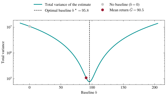
In the plot, the parabola is real, on a logarithmic vertical axis so both arms fit in the frame: the variance at the optimal baseline \(b^\star\) sits orders of magnitude below the variance at \(b = 0\), and the plain mean return \(\bar{G}\), the one baseline an agent can estimate for free while it trains, captures nearly all of that reduction.
One number served every state the agent visited, and states are not interchangeable.
The Advantage
Par should depend on where you are: from a balanced pole, a return of \(80\) is routine; from a pole about to topple, the same \(80\) is a miracle. A good baseline, like a good golf course, sets par hole by hole: here, state by state.
Problem 23 built the first object we need, the value function; the second, the Q-function, refines it by fixing the agent’s first action: \[ V^\pi(s) = \mathbb{E}[G_t \mid s_t = s], \qquad Q^\pi(s, a) = \mathbb{E}[G_t \mid s_t = s, \, a_t = a]. \] In words, \(V^\pi(s)\) is the expected return from state \(s\) under the current policy, and \(Q^\pi(s,a)\) fixes the first action to \(a\) and follows the policy afterward. Their difference is the advantage: \[ A^\pi(s, a) = Q^\pi(s, a) - V^\pi(s), \] how much better (or worse) action \(a\) is than the policy’s par from state \(s\). Because \(V^\pi(s) = \mathbb{E}_{a \sim \pi(\cdot|s)}[Q^\pi(s,a)]\), the advantage averages to exactly zero at every state: \[ \mathbb{E}_{a \sim \pi(\cdot|s)}\left[A^\pi(s,a)\right] = \mathbb{E}_{a \sim \pi(\cdot|s)}\left[Q^\pi(s,a)\right] - V^\pi(s) = 0. \] A positive advantage beat the policy’s own average from that state and a negative one fell short, so good and bad actions finally push in opposite directions instead of merely with different force. Practical algorithms weight each step’s score \(\nabla_{\boldsymbol\theta} \log \pi_{\boldsymbol\theta}(a_t|s_t)\) by an estimate of \(A^\pi(s_t, a_t)\), typically the observed return minus an estimate of \(V^\pi(s_t)\). (Learning \(\widehat{V}\) with a second network alongside the policy is the actor–critic family of algorithms.)
Is \(V^\pi(s)\) the variance-optimal state-dependent baseline? Very nearly, and the gap is Problem 25’s business: you will redo today’s minimization with \(b\) free to vary per state, derive the true optimum \(b^\star(s)\), and argue that \(V^\pi(s)\) is the approximation every practical algorithm rightly settles for. The value function is almost the perfect control variate, state by state.
Mean-Centering Across a Batch
The theory compresses into a two-line recipe that most implementations use verbatim. Run a batch of \(N\) episodes with the current policy, compute their returns \(G^{(1)}, \ldots, G^{(N)}\), and weight each episode’s score by the centered return in place of the raw one: \[ G^{(i)} - \bar{G}, \qquad \bar{G} = \frac{1}{N} \sum_{j=1}^N G^{(j)}. \] The batch estimates its own baseline, at zero extra cost. (In practice the centered returns are usually also divided by the batch’s standard deviation, which makes the update immune to the reward’s scale as well as its shift. Watch that denominator: once every episode in a batch returns the same number, the standard deviation is zero and the division amplifies floating-point dust into garbage weights.) This is the sample version of subtracting \(\mathbb{E}[G]\), the same baseline the parabola showed captures nearly all of the optimal reduction. The class demo reruns REINFORCE on CartPole three times, changing only the number that multiplies the score, and replays Problem 24’s bonus scandal live to confirm mean-centering erases it entirely.
A Leash on the Update
Variance is the noise within one update; a second danger lives between updates, and it is special to reinforcement learning. A too-aggressive step in supervised learning damages the model but not the data, since the dataset sits still. Here the policy is the data source, so an update that wrecks the policy also wrecks the experience collected next, and the agent may never see the states that would teach it to recover; that is what happened in last lecture’s collapse to a return of \(9\), where the network destroyed the behavior generating its own curriculum.
The remedy is to measure an update’s size in behavior space rather than parameter space, and the ruler is one we met in the Logistic Regression lecture: the KL divergence. Trust-region methods constrain each update to keep the new policy within a KL budget \(\delta > 0\) of the old one: \[ \mathbb{E}_s\left[\textnormal{KL}\big(\pi_{\text{old}}(\cdot|s) \,\|\, \pi_{\text{new}}(\cdot|s)\big)\right] \leq \delta. \] Read the constraint as a leash: the policy may improve as fast as it likes, as long as its behavior on the states it visits stays close to what it was. PPO, proximal policy optimization, enforces the same idea more cheaply by clipping the objective once the new policy strays too far. The leash appears one more time when a chatbot is fine-tuned from human feedback (RLHF), where the objective is the expected reward minus \(\beta \, \textnormal{KL}(\pi_{\boldsymbol\theta} \,\|\, \pi_{\text{ref}})\), with \(\beta > 0\) setting the leash’s tightness and \(\pi_{\text{ref}}\) the pretrained transformer itself. The model is rewarded for pleasing human preferences but tethered to the language model it started as, because an unconstrained policy drifts into gibberish that games the reward. Assemble this unit’s pieces, a policy gradient plus advantage-weighted updates plus a KL leash, and you have PPO as used in RLHF: the algorithm that finished training the chatbots is, nearly line for line, this lecture.
Closing the Course
There is no next lecture to hand off to, so let’s look back. Thirteen weeks ago the course opened with dice, and four threads have run through everything since.
- Variance reduction. Problem 1 proved that correlation puts a floor under averaging. Lecture two turned correlation into a tool, the control variate, and Problem 2 found its optimal coefficient \(\textnormal{Cov}(f,g)/\textnormal{Var}(g)\). Stochastic gradient descent turned out to be a Monte Carlo estimator whose variance sets the learning rate. And today the policy-gradient baseline turned out to be that same coefficient.
- MLE and Bayes. A Gaussian noise model made squared error inevitable, Bayes’ rule built the sigmoid, priors became regularizers, and REINFORCE turned out to be maximum likelihood on the agent’s own actions, weighted first by the return and as of today by the advantage.
- The SVD and spectra. The power method’s eigengap clock, the condition number that governs gradient descent, Eckart–Young–Mirsky, PCA, LoRA’s low-rank updates, and Muon’s singular-value surgery: one decomposition doing real work in six different lectures.
- Structure. Convolution is a matrix that commutes with shift, and attention’s rotary embeddings make the score matrix Toeplitz. Both are a symmetry written into the weights.
The through-line is the first one: on the second day of class we said that an unbiased estimator’s quality is its variance, and that cleverness rather than more samples brings the variance down; that cleverness now steadies the algorithm that fine-tunes frontier language models. To learn an average, take an average; to learn it well, subtract what you already know. One problem remains: Problem 25 hands you the bandit whose scandal started this, and the formula that ends it. The variance-reduction thread that opened the course closes it.