Contrastive Learning
Motivation
In the supervised learning setting, we train a neural network to predict the labels of points. Crucially, we need lots and lots of labelled data to get a network that works well. Unfortunately, it can be infeasible to acquire labels. In the particular example we consider today, we imagine that we have many images but we cannot afford to have them all labelled. Fortunately, we can still apply our deep learning toolkit to do something useful with the unlabelled images. The something is contrastive learning: We embed the images in a latent space that captures the important features of each image. Then, when we have a downstream task on the images, we train another network that uses the embeddings of the images instead of the images themselves. Since the embeddings are so meaningful, the network can use fewer weights and fewer labels than we’d otherwise need.
Set up
Suppose we have lots of images but no idea what each image depicts. Nonetheless, we persevere and embed the images into a latent space. Formally, consider a neural network \(f_{\pmb{\theta}} : \mathbb{R}^{a \times b \times c} \rightarrow \mathbb{R}^k\) that maps the \(a \times b \times c\)-dimensional images into \(k\)-dimensional vectors. What makes some embeddings (i.e. the parameters \(\pmb{\theta}\)) better than others? Well, we would really like for the embeddings of two images to be close if the two images depict similar content. Now notice this problem would be easier if we had labels telling us the content of each image: We could ensure two embeddings are close if they come from images with the same label and far otherwise. But, because we don’t have labels, we’ll need to be more clever in finding images of similar content.
Instead of embedding the images directly, suppose we augment the images by cropping, blurring, rotating, or any other method you can imagine. Then, we embed the augmented images. Formally, if \(\mathbf{x}\) is the augmented image, then we say \(f_{\pmb{\theta}}(\mathbf{x})\) is an embedding of the augmented image. Presumably, our augmented images still look like actual images we might come across in the wild but now we know if two images depict the same content without anyone giving us labels.
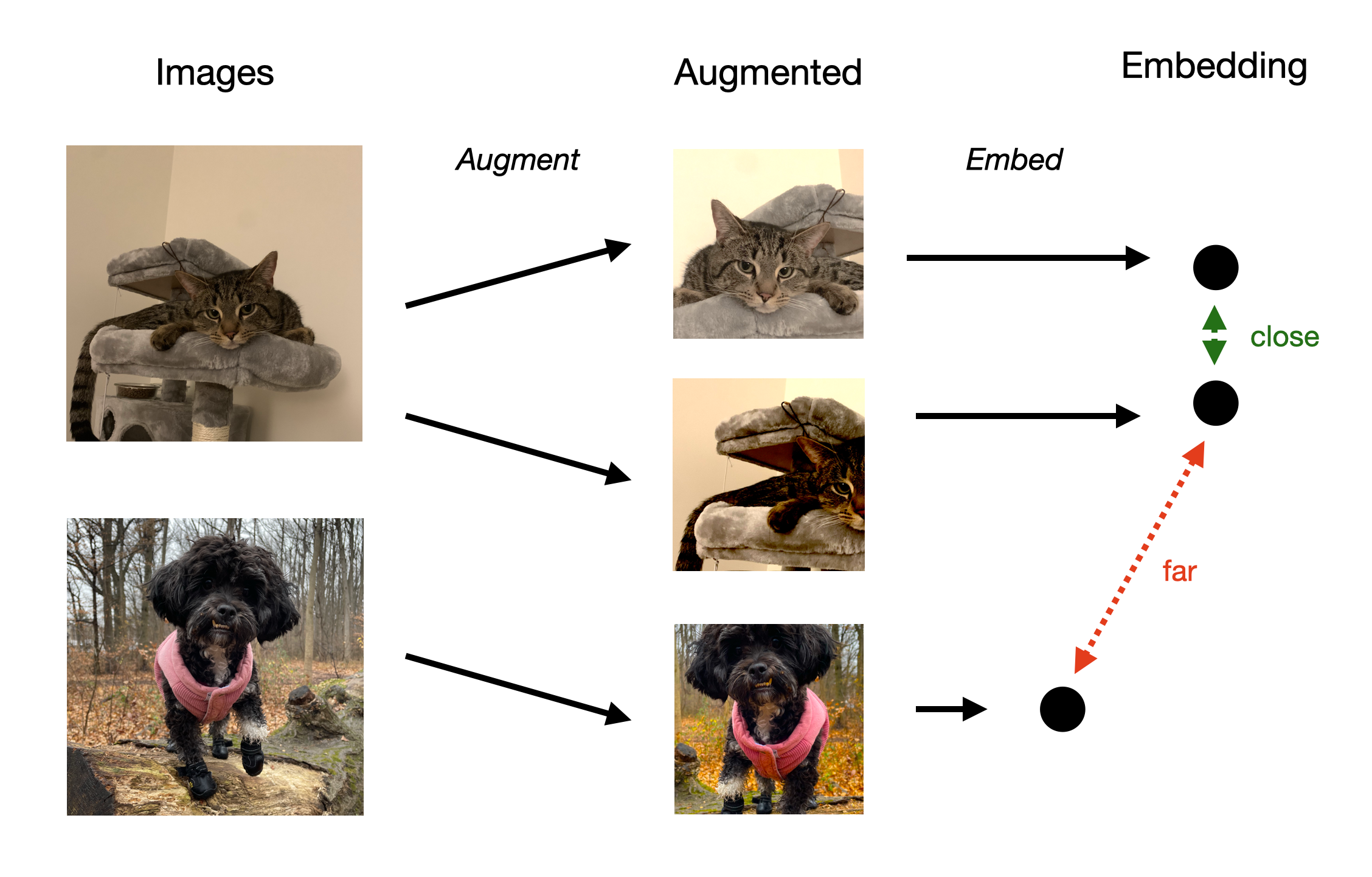
In the example figure above, we augment an image of Stripes and an image of Marley and embed the augmented images with our network. We would like for the embedded augmentations of Stripes to be close (since they have similar content) and the embedded augmentation of Marley to be far (since it has different content).
To make our embeddings meaningful, let’s turn to our three-step recipe for deep learning. We have our architecture \(f_{\pmb{\theta}}\) and trusty optimizer stochastic gradient descent. What should our loss be?
Loss Functions
It turns out there are many choices of loss functions for contrastive learning. If you are feeling particularly indomitable, check out Lilian Weng’s impressively comprehensive blog post here. Today, we’ll consider one of the most straightforward.
This loss function is intuitively motivated: We want the distance between two embedded augmentations of the same image to be small while the distance between two embedded augmentations of different images to be large. Since they are vectors, a natural choice of distance between embeddings is their inner product. In general settings, we say two points form a positive pair if they are similar and a negative pair if they are not. Of course, we want this property to hold on average for all pairs of embedded augmentations. Formally, we can put these constraints in the following loss function as \[\mathcal{L}(\pmb{\theta}) = -2 \mathbb{E}_{\mathbf{x, x}' \sim \textrm{positive}} [f_{\pmb{\theta}}^\top(\mathbf{x}) f_{\pmb{\theta}}(\mathbf{x}')] + \mathbb{E}_{\mathbf{x, x'} \sim \textrm{negative}} [(f_{\pmb{\theta}}^\top(\mathbf{x}) f_{\pmb{\theta}}(\mathbf{x}'))^2].\]
Since we train the parameters to minimize the loss, we’ll (hopefully) end up with a small loss. By design, a small loss corresponds to the relationship we want between pairs: The first term is negative when the embeddings of positive pairs have large inner product and the second term is close to zero when the embeddings of negative pairs have small inner product in absolute value. Notice that we square the inner product of the negative pairs so that the second term is always non-negative; otherwise, the network could cheat by making the inner product very negative.
Applications
We now have an architecture, loss function, and optimizer in hand. What can we do with them? There are two applications we’ll discuss.
The first application is linear regression on top of the embeddings. Suppose that we managed to label some (but definitely not all or most) of our images with binary labels like “cat” and “dog”. We tried to train a standard neural network on the images to predict the labels but we got poor validation accuracy because we had too few labelled images and/or not enough compute. Instead, we turn to contrastive learning to train a network \(f_{\pmb{\theta}}\) for embedding the unlabelled images.
Now, with the embeddings of the few labelled images we have, we train a linear regression model to predict the label. Remember that linear regression is equivalent to training a neural network with a single neuron. I want to emphasize that this approach is the antithesis of modern deep learning: We use very limited resources to train a very simple model. Indeed, it should be surprising that this approach could work at all because images are quite complicated and we typically need lots of fancy convolutional layers to process them. But, not only does linear regression suffice, we can actually prove that we achieve low loss that depends on properties of the data. In fact, the proof appears at the end of these notes.
The second application is Contrastive Language-Image Pre-training (CLIP). The idea is that we want to embed images and text into the same latent space so that two embeddings are close if the original text describes the original image. The key insight of CLIP is carefully defining positive pairs: We say an image and a text description form a positive pair if the text describes the image. How do we find such nice data? Well, we crawl the web and use all the text descriptions people have created for the images they post. Then we carry on with contrastive learning as we did before: We encourage embeddings of positive pairs to be close and embeddings of negative pairs to be far.
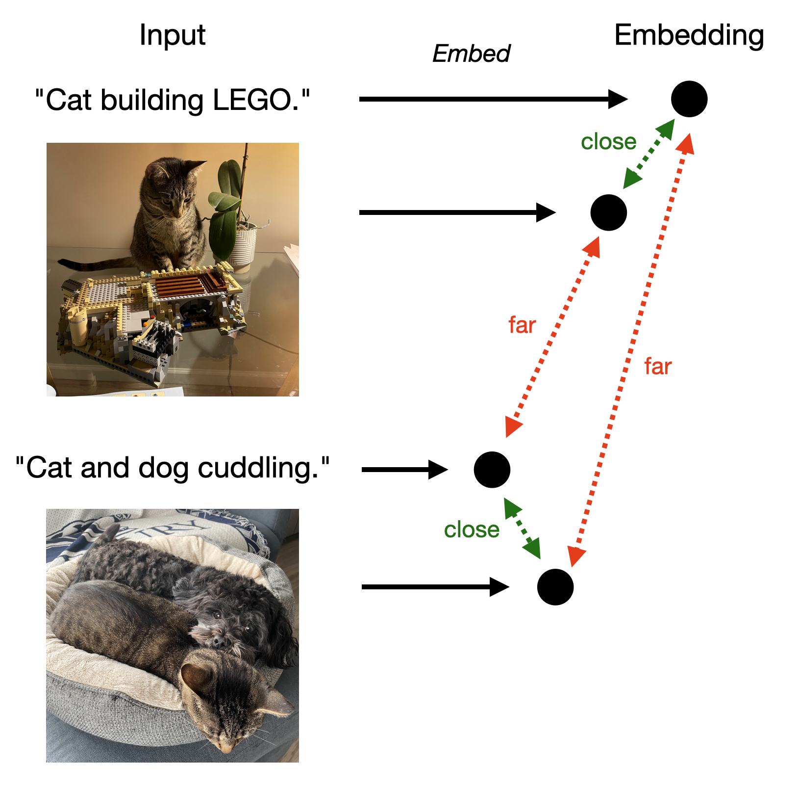
The process is illustrated in the figure above. Of course, we’ll need one model to embed the images and another NLP model to embed the text. Once we trained two working models for CLIP, we can run diffusion in the embedded latent space conditioned on the text description. This technique forms the backbone of stable diffusion. In addition, we can use CLIP to search for images by embedding a text description and finding images with similar embeddings. Or, we can even search for text by embedding an image and finding text with similar embeddings.
Debiasing
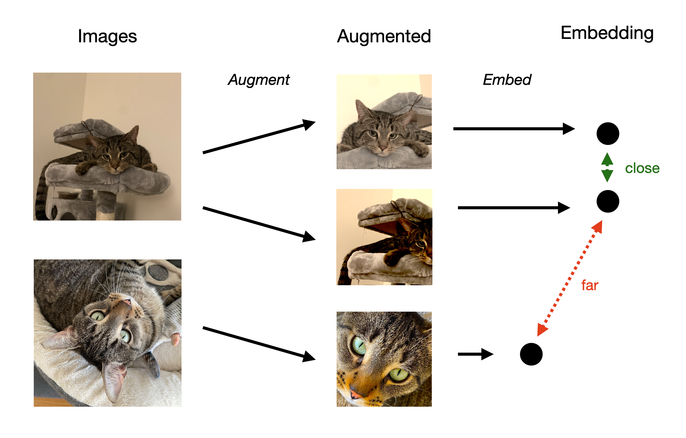
So far, we’ve ignored a pesky problem with contrastive learning. What if a negative pair is actually a positive pair? For concreteness, let’s return to the augmented image setting to articulate the issue. Suppose we have two different images of Stripes but, because there are no labels, we don’t know the images depict the same cat. Then, when we train our embedding network, we force two embedded augmentations of Stripes apart which reduces the quality of the latent space. The current behavior of contrastive learning is illustrated below.
Fortunately, we can correct the problem with a different contrastive loss function and some clever math. In order to motivate the new loss function, suppose we have fixed an augmented image \(\mathbf{x}\) and we’re sampling for a positive partner \(\mathbf{x}^+\). Let \(\Pr(\mathbf{x}^+ | \mathbf{x})\) be the probability that we sample a particular positive partner \(\mathbf{x}^+\). Similarly, let \(\Pr(\mathbf{x}^-| \mathbf{x})\) be the probability that we sample a particular negative partner \(\mathbf{x}^-\).
How do we perform this sampling? Well, we look around the embedding of our “anchor” \(\mathbf{x}\) and sample an image \(\mathbf{x'}\) with probability proportional to the exponentiated distance between the embeddings of \(\mathbf{x}\) and \(\mathbf{x'}\). Formally, \(\Pr(\mathbf{x}' | \mathbf{x}) \propto \exp(f_{\pmb{\theta}}(\mathbf{x})^\top f_{\pmb{\theta}}(\mathbf{x}'))\). Notice that we’re simply taking the softmax of the distances here. Now one way to encourage the distance between positive pairs to be small and negative pairs to be large is to use the loss given by
\[ \mathcal{L}(\pmb{\theta}) = \mathbb{E}_{\mathbf{x}, \mathbf{x}^+, \mathbf{x}^-} \left[ - \log \left( \frac{\Pr(\mathbf{x}^+ | \mathbf{x})} {\Pr(\mathbf{x}^+ | \mathbf{x}) + \Pr(\mathbf{x}^- | \mathbf{x})}\right)\right]. \]
Somewhat surprisingly, we can show that this contrastive loss is equivalent up to constants with our first contrastive loss. (As my undergraduate advisor Bill Peterson used to say, “What’s a constant between friends?”.) To preserve the mystique, we’ll leave this proof as an exercise for the motivated reader.
With our shiny new (but really the same) loss function, we can articulate the pesky problem as using a biased estimate for \(\Pr(\mathbf{x}^- | \mathbf{x})\) because sometimes \(\mathbf{x}\) and \(\mathbf{x}^-\) are actually a positive pair. Fortunately, we can replace our biased estimate with an unbiased estimate.
Once we fix an image \(\mathbf{x}\), the law of total probability tells us that the probability we sample a particular image is given by
\[ \Pr(\mathbf{x}' | \mathbf{x}) = \eta \Pr ( \mathbf{x}' | y = y', \mathbf{x} ) + (1-\eta) \Pr (\mathbf{x}' | y \neq y', \mathbf{x}) \] where \(\eta\) is the probability we draw an image from a different class than that of \(\mathbf{x}\) and \(y\) is the label of \(\mathbf{x}\). Rearranging and simplifying, we can write \[ \Pr(\mathbf{x}^- | \mathbf{x} ) = \frac{\Pr(\mathbf{x}' | \mathbf{x})}{1-\eta} - \eta \frac{\Pr(\mathbf{x^+}| \mathbf{x})}{1-\eta}. \] We now have a more complicated expression for \(\Pr(\mathbf{x}^-|\mathbf{x})\) but we have an unbiased estimate for each term: We can estimate \(\eta\) based on what we expect from the distribution of the data. We can estimate \(\Pr(\mathbf{x}^+|\mathbf{x})\) with Monte Carlo sampling because we reliably identify positive pairs. We can estimate \(\Pr(\mathbf{x}'|\mathbf{x})\) with Monte Carlo sampling since we don’t require labels to do so. As a result, we plug our new unbiased estimate into the loss function as a replacement for the biased estimate. We call the resulting loss function debiased.
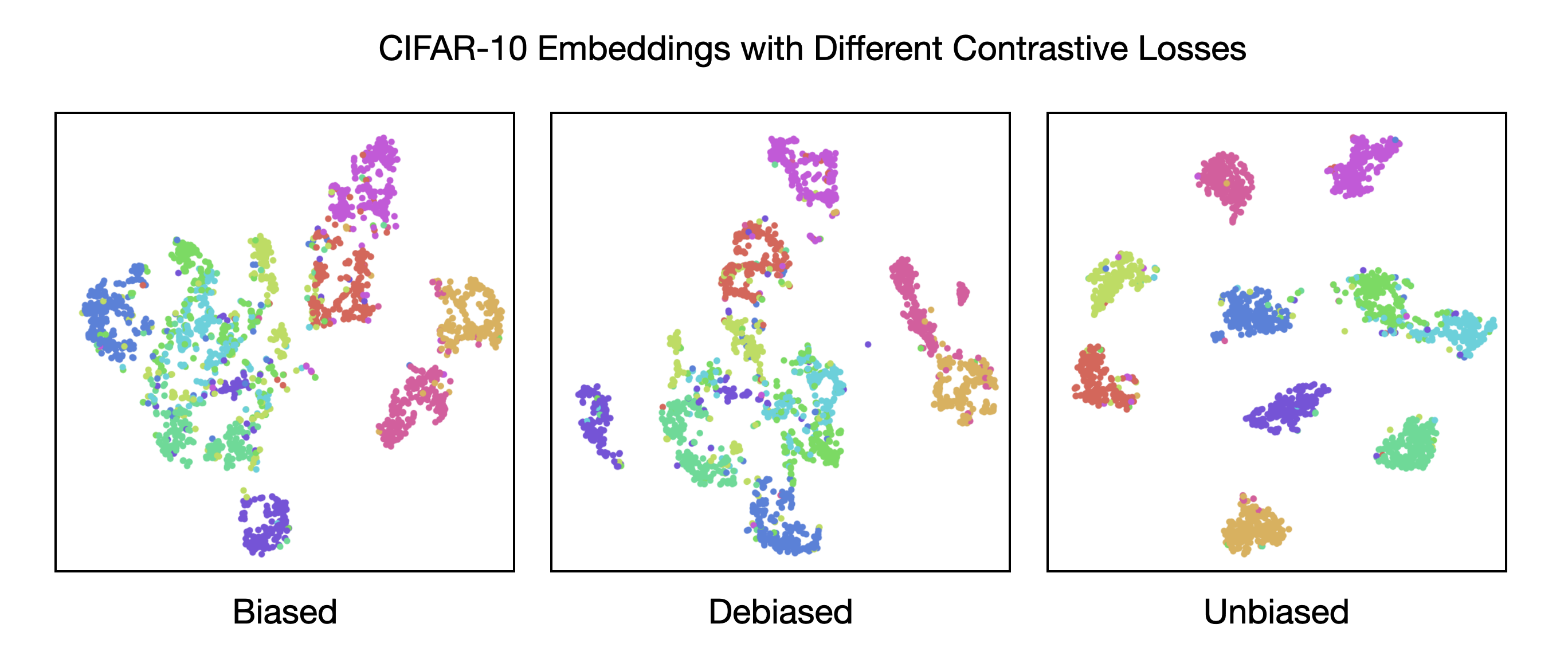
The below figure illustrates the difference in the quality of the embedded clusters between using the biased version of the loss function, the debiased version, and the unbiased version (where we use true labels to eliminate false negative pairs).
Optional: Provable Guarantees for Contrastive Learning
Recall the first contrastive learning loss given by:
\[\mathcal{L}(\pmb{\theta}) = -2 \mathbb{E}_{\mathbf{x, x}' \sim \textrm{positive}} [f_{\pmb{\theta}}^\top(\mathbf{x}) f_{\pmb{\theta}}(\mathbf{x}')] + \mathbb{E}_{\mathbf{x, x'} \sim \textrm{negative}} [(f_{\pmb{\theta}}^\top(\mathbf{x}) f_{\pmb{\theta}}(\mathbf{x}'))^2]\]
The first term ensures that embeddings of positive pairs (augmentations of the same image) are close while the second term ensures that embeddings of negative pairs (augmentations of different images) are far.
Once we train the network \(f_{\pmb{\theta}}\) on this loss, we will use use the embeddings for the downstream task of predicting binary labels of images. Amazingly, because of the meaning captured in the embeddings, we can label the images using only linear regression (i.e. a single neuron). We will use the following loss function for the downstream task:
\[\mathcal{L}_\textrm{task}(\mathbf{w}, \pmb{\theta}) = \mathbb{E}_{\mathbf{x},y}[(y - \mathbf{w}^\top f_{\pmb{\theta}}(\mathbf{x}))^2]\] where the expectation is over a (small) number of images \(\mathbf{x}\) with labels \(y\).
Generally, we do not know how to prove that deep learning techniques work. Contrastive learning is a notable exception. By combining ideas from spectral graph theory and linear algebra, we will be able to show (under several assumptions) that we can find good parameters for the contrastive learning task we have set up so far. The proof we present is based on notes (section 10.3) from Tengyu Ma’s phenomenal machine learning theory class.
Proof Structure
We want to show that the parameters we find from training give a loss that is very small. Along the way, there are several sources of error that we need to handle:
We train on samples drawn from a distribution so the empirical loss we work with is not quite the true loss.
We use gradient descent to find good parameters but we might not get exactly the true minimizer to the empirical loss.
It is possible the optimal parameters of the true loss do not give a good solution thus our parameters can’t give a good solution either.
We will wave our hands at the first two problems and dive into the third. In particular, we will assume the empirical loss function approximates the true loss given enough samples. In addition, we will assume that gradient descent converges to the minimizer of the empirical loss function. With these assumptions, we can bound the error of our parameters.
Suppose that we train on the contrastive loss first and, sweeping several issues under the rug, find \[\pmb{\theta}^* = \arg \min_{\pmb{\theta}} \mathcal{L}(\pmb{\theta}).\]
Now, we fix \(\pmb{\theta}^*\) and train on the task loss to find \(\mathbf{w}\). Let \(\mathbf{w}^*\) be the optimal solution on the true task loss and \(\hat{\mathbf{w}}\) be the solution we find by training on the empirical task loss. Formally, we have
\[\hat{\mathcal{L}}_\textrm{task}(\hat{\mathbf{w}}, \pmb{\theta}^*) = \min_{\mathbf{w}} \hat{\mathcal{L}}_\textrm{task}(\mathbf{w}, \pmb{\theta}^*) \le \hat{\mathcal{L}}_\textrm{task}(\mathbf{w}^*, \pmb{\theta}^*) \le \mathcal{L}_\textrm{task}(\mathbf{w}^*, \pmb{\theta}^*) + \epsilon.\]
The first equality follows by our assumption on gradient descent, the first inequality follows by the definition of the minimum, and the final inequality follows by our assumption that the empirical loss approximates the true loss.
Now it remains to show that the solution of the optimal parameters is small enough.
Graph Formulation
Consider a weighted and undirected graph on \(n\) nodes and \(m\) edges where each node corresponds to an augmented image. Two nodes share an edge if and only if they both are augmentations of the same original image. Let \(p(\mathbf{x}, \mathbf{x'})\) be the probability density of positive pair \(\mathbf{x}\) and \(\mathbf{x}'\). The weight of an edge is \(p(\mathbf{x}, \mathbf{x}')\).
Let \(\mathbf{A} \in \mathbb{R}^{n \times n}\) be the adjacency matrix and \(\mathbf{D} \in \mathbb{R}^{n \times n}\) be the degree matrix. We define the symmetric normalized matrix \(\bar{\mathbf{A}} = \mathbf{D}^{-1/2} \mathbf{A} \mathbf{D}^{-1/2}\). In particular,
\[\bar{\mathbf{A}}_{\mathbf{x}, \mathbf{x'}} = \frac{p(\mathbf{x}, \mathbf{x'})}{\sqrt{p(\mathbf{x}) p(\mathbf{x'})}}\]
where \(p(\mathbf{x}) = \sum_{\mathbf{x}'} p(\mathbf{x}, \mathbf{x}').\)
The first (very cool) observation is that we can exactly characterize the solution to the contrastive loss function.
Let \(\mathbf{F} \in \mathbb{R}^{n \times k}\) be the weighted embeddings where the \(i\)th row is \(\sqrt{p(\mathbf{x}_i)} f_{\pmb{\theta}}(\mathbf{x}_i)^\top\). Then
\[ \arg \min_{\pmb{\theta}} \mathcal{L}(\pmb{\theta}) = \arg \min_{\pmb{\theta}} \| \bar{\mathbf{A}} - \mathbf{F} \mathbf{F}^\top \|_F^2.\]
To see this, we write \[ \displaylines{\| \bar{\mathbf{A}} - \mathbf{F} \mathbf{F}^\top \|_F^2 = \sum_{\mathbf{x}, \mathbf{x'}} \left( \frac{p(\mathbf{x}, \mathbf{x'})} {\sqrt{p(\mathbf{x}) p(\mathbf{x'})}} - f_{\pmb{\theta}}(\mathbf{x})^\top f_{\pmb{\theta}}(\mathbf{x'}) \sqrt{p(\mathbf{x})} \sqrt{p(\mathbf{x'}}) \right)^2 \\ = \textrm{constant} - 2 \sum_{\mathbf{x, x'}} p(\mathbf{x}, \mathbf{x'}) f_{\pmb{\theta}}(\mathbf{x})^\top f_{\pmb{\theta}}(\mathbf{x}) + \sum_{\mathbf{x, x'}} p(\mathbf{x}) p(\mathbf{x'}) \left(f_{\pmb{\theta}}(\mathbf{x})^\top f_{\pmb{\theta}}(\mathbf{x}) \right)^2 \\ = \textrm{constant} -2 \mathbb{E}_{\mathbf{x, x}' \sim \textrm{positive}} [f_{\pmb{\theta}}^\top(\mathbf{x}) f_{\pmb{\theta}}(\mathbf{x}')] + \mathbb{E}_{\mathbf{x, x'} \sim \textrm{negative}} [(f_{\pmb{\theta}}^\top(\mathbf{x}) f_{\pmb{\theta}}(\mathbf{x}'))^2].}\]
Notice that the last two terms are exactly the contrastive loss \(\mathcal{L}(\pmb{\theta})\). This observation is incredibly helpful since we know how to find the optimal \(\mathbf{F}\): We want the best rank \(k\) approximation which is \(\mathbf{F} \mathbf{F}^\top = \mathbf{U}_k \mathbf{\Lambda}_k \mathbf{U}_k^T\) where the columns of \(\mathbf{U}_k\) are the top \(k\) eigenvectors of \(\bar{\mathbf{A}}\) and the (diagonal) entries of \(\mathbf{\Lambda}_k\) are the top \(k\) eigenvalues. Let \(\mathbf{u}_i^\top\) be the \(i\)th row of \(\mathbf{U}_k\). Then \(f_{\pmb{\theta}^*}(\mathbf{x}_i) = p(\mathbf{x}_i)^{-1/2} \mathbf{\Lambda}_k^{1/2} \mathbf{u}_i\).
We have found the optimal embeddings but we still need to show we can achieve good performance on the task loss.
Bounding the Task Loss
In order to say something interesting about the task loss, we’ll need a few more assumptions about our graph.
Suppose the graph is \(\kappa\) regular. That is, \(p(\mathbf{x}) = \sum_{\mathbf{x}'} p(\mathbf{x}, \mathbf{x}') = \kappa\) for all \(\mathbf{x}\). In our context, this means each image is equally likely to be chosen.
Suppose the graph can be well separated into two sets. In our context, this means half the images depict dogs while the other half depict cats. Formally, we assume there exists a set of vertices \(S\) with \(|S| = n/2\) so that \(E(S, \bar{S}) = \sum_{\mathbf{x} \in S, \mathbf{x}' \in S} p(\mathbf{x}, \mathbf{x}') \le \alpha \kappa n\) for some \(\alpha \in (0,1)\).
Suppose the graph cannot be well separated into three non-empty sets. In our context, this means there is no good alternative way of classifying images of cats and dogs (e.g. wearing shoes, sitting down, eating). Formally, we assume for all partitions \(S_1, S_2, S_3\) that \[\max_{i \in \{1,2,3\}} \frac{E(S_i, \bar{S_i})}{p(S_i)} \ge \rho\] where \(p(S_i) = \sum_{\mathbf{x} \in S_i} p(\mathbf{x})\) and \(\rho \in (0,1)\).
Under these assumptions, we will show that
\[\mathcal{L}_\textrm{task}(\mathbf{w}^*, \pmb{\theta}^*) = \frac{1}{n} \sum_{i=1}^n (y_i - {\mathbf{w}^*}^\top f_{\pmb{\theta}^*}(\mathbf{x}_i))^2 \lesssim \frac{\alpha}{\rho^2}\] where the approximate inequality hides constants.
Define \(\mathbf{L}\) as the normalized Laplacian of the graph \(\mathbf{I} - \bar{\mathbf{A}}\). Let \(\lambda_1 \le \lambda_2 \le \ldots \le \lambda_n\) be the eigenvalues of \(\mathbf{L}\) and \(\mathbf{v}_1, \mathbf{v}_2, \ldots, \mathbf{v}_n\) be the corresponding eigenvectors. Notice that \(\mathbf{L}\) and \(\bar{\mathbf{A}}\) share eigenvectors; in particular, the \(k\) smallest eigenvectors of \(\mathbf{L}\) are the same as the top \(k\) eigenvectors \(\bar{\mathbf{A}}\).
We will need the following technical ingredient.
Key Lemma [Proposition 1.2 in Louis and Makarychev]: Suppose for all partitions of nodes into \(\ell\) non-empty sets \(S_1, \ldots, S_\ell\), we have \[\max_{i \in [\ell]} \frac{E(S_i, \bar{S_i})}{p(S_i)} \ge \rho.\] Then \(\rho^2 \lesssim \lambda_{2\ell}\) where the hidden constant depends on \(\log(\ell)\).
We will begin by analyzing \(\mathbf{y}^\top \mathbf{L} \mathbf{y}\). Recall that we can write \(\mathbf{L}=\mathbf{B}\mathbf{W}\mathbf{B}^\top\) where \(\mathbf{B} \in \mathbb{R}^{n \times m}\) is the edge incidence matrix and \(\mathbf{W} \in \mathbb{R}^{m \times m}\) is the normalized edge weight matrix. In particular, each column of \(\mathbf{B}\) corresponds to a positive pair \((\mathbf{x}, \mathbf{x}')\) with +1 in the row corresponding to \(\mathbf{x}\) and -1 in the row corresponding to \(\mathbf{x}'\) (or vice versa). With this observation, we can write
\[\mathbf{y}^\top \mathbf{L y} = \sum_{\mathbf{x}, \mathbf{x}'} (y - y')^2 \frac{p(\mathbf{x}, \mathbf{x}')}{\kappa} = \frac{2}{\kappa} \sum_{\mathbf{x} \in S, \mathbf{x'} \in \bar{S}} p(\mathbf{x}, \mathbf{x}') = \frac{2}{\kappa} E(S, \bar{S}) \le 2 \alpha n.\]
Suppose \(\mathbf{y} = \sum_{i=1}^n \beta_i \mathbf{v}_i\) for scalars \(\beta_i = \mathbf{y}^\top \mathbf{v}_i\). We will apply the lemma with \(2 \ell = k = 6\). We bound \[\sum_{i=k+1}^n \beta_i^2 \rho^2 \lesssim \sum_{i=k+1}^n \beta_i^2 \lambda_i \le \sum_{i=1}^n \beta_i^2 \lambda_i = \mathbf{y}^\top \mathbf{L y} \le 2\alpha n\] where the final inequality used that the \(\mathbf{v}_i\) are eigenvectors of \(\mathbf{L}\).
Choose \(\mathbf{w}\) and \(\pmb{\theta}\) so that \(f_{\pmb{\theta}}(\mathbf{x}_i) = p(\mathbf{x}_i)^{-1/2} \mathbf{\Lambda}_k^{1/2} \mathbf{u}_i = \kappa^{-1/2}\mathbf{\Lambda}_k^{1/2} \mathbf{u}_i\) and \(\mathbf{w} = \kappa^{1/2} \mathbf{\Lambda}_k^{-1/2} \pmb{\beta}\).
Plugging into the true task loss, we then have that
\[\displaylines{ \mathcal{L}_\textrm{task}(\mathbf{w}^*, \pmb{\theta}^*) = \frac{1}{n} \sum_{i=1}^n (y_i - {\mathbf{w}^*}^\top f_{\pmb{\theta}^*}(\mathbf{x}_i))^2 \le \frac{1}{n} \| \mathbf{y} - \sum_{i=1}^k \beta_i \mathbf{v}_i \|_2^2 \\ = \frac{1}{n} \| \sum_{i=k+1}^n \beta_i \mathbf{v}_i \|_2^2 = \frac{1}{n} \sum_{i=k+1}^n \beta_i^2 \lesssim 2 \frac{\alpha}{\rho^2}.}\]
We have shown there exist parameters that give
• the optimal solution to the true contrastive loss and
• a data-dependent bound on the true task loss.
Finally, putting it all together, we have that the parameters we find through training on the empirical task loss satisfy \[\mathcal{\hat{L}}(\hat{\mathbf{w}}, \hat{\pmb{\theta}}) \lesssim \frac{\alpha}{\rho^2} + \epsilon.\]