Stable Diffusion
Motivation
We previously discussed generative adversarial networks (GANs). GANs create realistic images by playing a game between a “generator” network and a “discriminator” network; the generator learns to create realistic images while the discriminator learns to differentiate between these fake images and the real ones. Unfortunately, GANs suffer from a problem called mode collapse. During training, the generator can memorize a single image from the real data set and the discriminator (correctly) determines that the image is real. The problem is that training stops because the generator has achieved minimum loss. Now, we’re stuck with a generator that only outputs one image (to be fair, the one image does look real).
There have been several attempts to mitigate mode collapse by trying different loss functions (a loss function based on Wasserstein distance is particularly effective) and adding a regularization term (the idea is to force the generator to use the random noise it’s given as input). However, these and similar approaches cannot completely prevent mode collapse.
So we’re left with the same problem we had before: how to generate realistic images. Instead of GANs, the deep learning community has recently turned to diffusion …and the results are astounding. The basic idea of diffusion is to repeatedly apply a de-noising process to a random state until it resembles a realistic image. Let’s dive into the details.
Diffusion Process
Our goal is to turn random noise into a realistic image. The starting point of diffusion is the simple observation that, while it’s not obvious how to turn noise into a realistic image, we can turn a realistic image into noise. In particular, starting from a real image in our data set we can repeatedly apply noise (typically drawn from a normal distribution) until the image becomes completely unrecognizable. Suppose \(x_0\) is the real image drawn from our data set. Let the first noised image be \(x_1 = x_0 + \epsilon_1\) where the noise \(\epsilon_1\) is drawn from a normal distribution \(\mathcal{N}(\mathbf{0}, \sigma^2 \mathbf{I})\) for a carefully chosen variance \(\sigma^2\). In this way, we can repeatedly generate \(x_{t} = x_{t-1} + \epsilon_{t}\) where \(\epsilon_{t} \sim \mathcal{N}(\mathbf{0}, \sigma^2 \mathbf{I})\). If we repeat for a carefully chosen number of steps \(T\), we now have a sequence \(x_0, x_1, \ldots, x_T\) such that the images become more and more similar to noise.
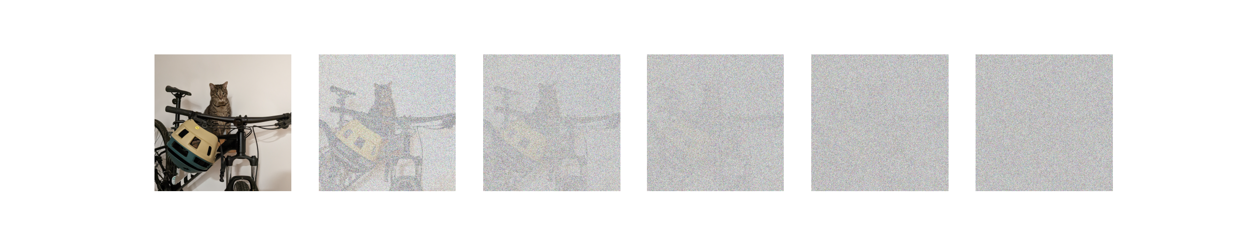
In this example, we made a picture of a cat on a bike completely unrecognizable by adding normal noise five times. The key insight is that if we look at this sequence backwards then we have training data which we can use to teach a model how to remove noise.
Formally, the training data consists of \(x_t\), \(t\), and \(x_{t-1}\). Our goal is to train a model \(f_\theta\) to predict \(x_{t-1}\) from \(x_t\) and \(t\). A very natural choice of loss function is then
\[\mathcal{L}(\theta) = \mathbb{E} [\| x_{t-1} - f_\theta(x_t, t) \|^2]\] where the expectation is over \(x_t\), \(t\), and \(x_{t-1}\). Unfortunately, unlike the noise itself, the noisy images are quite variable. As a result, researchers have found that the process is more stable if \(f_\theta\) predicts the noise \(\epsilon_{t}\) and then we compute \(x_{t-1} = x_t - \epsilon_t\). Formally, the loss function is
\[\mathcal{L}(\theta) = \mathbb{E} [\| \epsilon_{t} - f_\theta(x_t, t) \|^2]\] where the expectation is again over \(x_t\), \(t\), and \(x_{t-1}\).
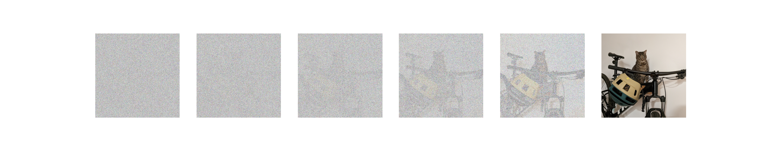
Once we have a working \(f_\theta\), we can use it to generate realistic images. We start with random noise which we’ll call \(x_T'\). Then for \(t=T,\ldots, 1\), we predict \(\epsilon_t' = f_\theta(x_t', t)\) and compute \(x_{t-1}' = x_t' - \epsilon_t'\). The final result \(x_0'\) is what the diffusion process outputs. With any luck, this output is a realistic image.
Thinking back to our three-step recipe for machine learning, we have the loss function and optimizer (SGD, as usual) but how do we choose an architecture? Since we’re working with images, a natural choice is a convolutional network. (In stable diffusion, the diffusion model is a convolutional network with residual connections.) However, even with convolutional layers, we will have a dependence between the size of the network and the size of the images. This presents a problem for us because we’d like to be able to train a diffusion model once and use it to produce both very high resolution images and very low resolution images. In other words, we’d like to run diffusion in a space whose dimension is independent of the size of the images. On its face, this seems quite hard but, as we’ll see, we can use autoencoders.
Autoencoders
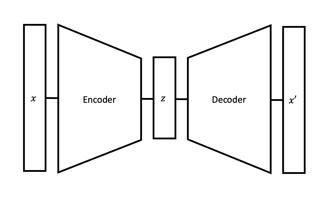
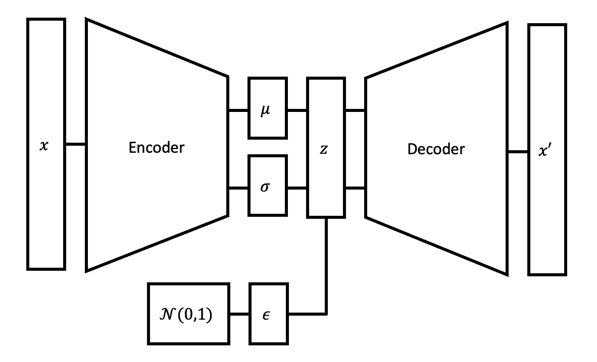
Autoencoders are a method for encoding images into a low-dimensional latent space. Once encoded in the latent space, we use a decoder to decode the image back to pixel space and recover an approximation of the original image. In mathematical notation, we have a starting image \(x\) and we use the encoder network to produce a latent representation \(z\). Then, using the decoder network we decode the latent representation \(z\) into an approximation of the original image \(x'\). In order to ensure that \(x\) and \(x'\) are close, we train the model with a reconstruction loss given by \[ \mathcal{L}_\text{reconstruction}(\Theta, \Omega) = \mathbb{E} [\| x - x' \|^2 ] \] where \(\Theta\) is the set of parameters in the encoder and \(\Omega\) is the set of parameters in the decoder.
Once trained, autoencoders tend to work quite well in the sense that the latent representation holds enough information to reconstruct the original image. So what do they have to do with diffusion? Well, we want to run the diffusing process in a dimension that is independent of the resolution of the image. Autoencoders can help if we encode the image and run diffusion in the latent space. Then, at test time when we generate a new image in the latent space, we can decode it back to pixel space.
Unfortunately, we hit a snag in the last step. Even though we know we can encode each image into the latent space and decode back to the pixel space, we don’t know that a random vector in the latent space will give us a nice image in the pixel space.
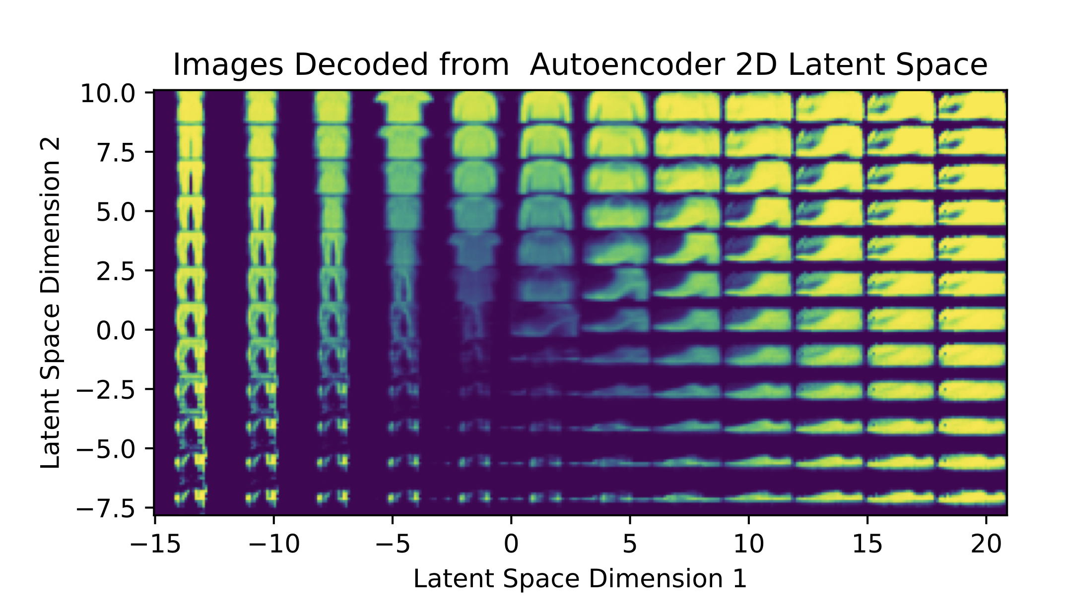
In the figure above, we sample vectors from a two dimensional latent space and decode the vectors back to pixel space. The autoencoder was trained on the FashionMNIST data set of clothing images. As we can see, images decoded from parts of the latent space are recognizable (e.g. some shoes in the middle) but the vast majority are not. As a result, autoencoders are not quite appropriate for diffusion because the latent representations generated from diffusion are not likely to have good pixel space decodings. Fortunately, variational autoencoders can help us.
Variational Autoencoders
Variational autoencoders are an extension of autoencoders with the property that encoded vectors are nicely distributed in the latent space. To ensure this property, variational autoencoders differ from standard autoencoders in two ways:
The variational encoder uses the starting image to produce a mean \(\mu\) and standard deviation \(\sigma\). The latent vector encoding is then generated by sampling from the normal distribution \(\mathcal{N}(\mu, \sigma^2)\). In contrast, the standard encoder deterministically produces a latent vector that only depends on the starting image and the encoder’s parameters.
We would like the mean and standard deviation produced by the variational encoder to be close to the unit normal distribution. In this way, the latent vectors will be distributed in the latent space “nicely”. We can ensure the two normal distributions are close by measuring the “distance” between \(\mathcal{N}(\mu, \sigma^2)\) and \(\mathcal{N}(0,1)\).
Before we develop this distance, let’s address a potential problem with the architectural modification. How do we backpropagate through a random sample? Honestly, I don’t know. But we can skirt around the issue by generating some random noise \(\epsilon\) from a unit normal distribution and computing latent vector as \(z = \mu + \sigma \epsilon\). When we backpropagate, the noise \(\epsilon\) is treated as a constant because, for a particular sample, it is a constant.
With the architecture fixed, we want a way of measuring the distance between two distributions, say \(P\) and \(Q\). Have we seen a loss for this task before? Yes! When we learned about image classification, we used the discrete cross entropy loss to measure the difference between our predicted classes and the true class.
We can use cross entropy again but, since we’re working with normal distributions, we’ll need the continuous version of cross entropy which we’ll call \(H(P,Q)\). (The discrete cross entropy uses a sum whereas the continuous cross entropy uses an integral.) Now, in order to make the loss a distance, we’d like the distance between \(P\) and \(P\) to be 0. However, the cross entropy of a distribution with itself is simply the entropy of the distribution which is in general not 0. To remedy this problem, we’ll simply subtract the entropy so that the variational loss is given by \[ \mathcal{L}_\text{variational}(\Theta) = H(P,Q) - H(P, P) \] where \(\Theta\) is the set of parameters in the variational autoencoder.
The variational loss we wrote down is known as the Kullback-Leibler divergence. The formula is complicated but, in the special case of \(P = \mathcal{N}(\mu, \sigma^2)\) and \(Q = \mathcal{N}(0,1)\), we have
\[ \mathcal{L}_\text{variational}(\Theta) = - \log(\sigma) + \frac{\sigma^2 + \mu^2 -1}{2}. \]
(You can find a derivation of the simplified equation here.)
Finally, with our modified architecture, we train on the combined loss \(\mathcal{L}_\text{reconstruction}(\Theta, \Omega) + \mathcal{L}_\text{variational}(\Theta).\) Of course, the question is whether our fancy variational autoencoder gives us any improvement. If we train a variational autoencoder on the FashionMNIST data set, we can make another plot of sampled latent vectors decoded to the pixels pace.
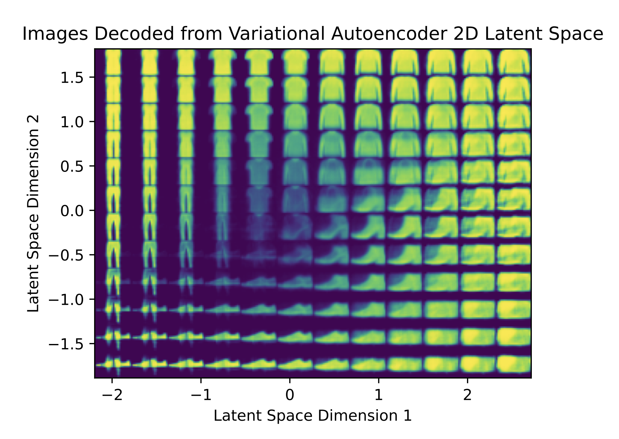
In the above figure, notice that the domain of the latent space is concentrated around 0 and, while not every decoded latent vector is discernible, they seem to be amalgamations of several clothing items. We conclude that the variational autoencoder is in fact better. Of course, if we want to get nicer decoded images, we’d likely need a latent space with more than two dimensions.
Stable Diffusion
Now that we understand the diffusion process and variational autoencoders, we’re ready to describe the stable diffusion pipeline. We will consider stable diffusion in the training and evaluation phases separately.
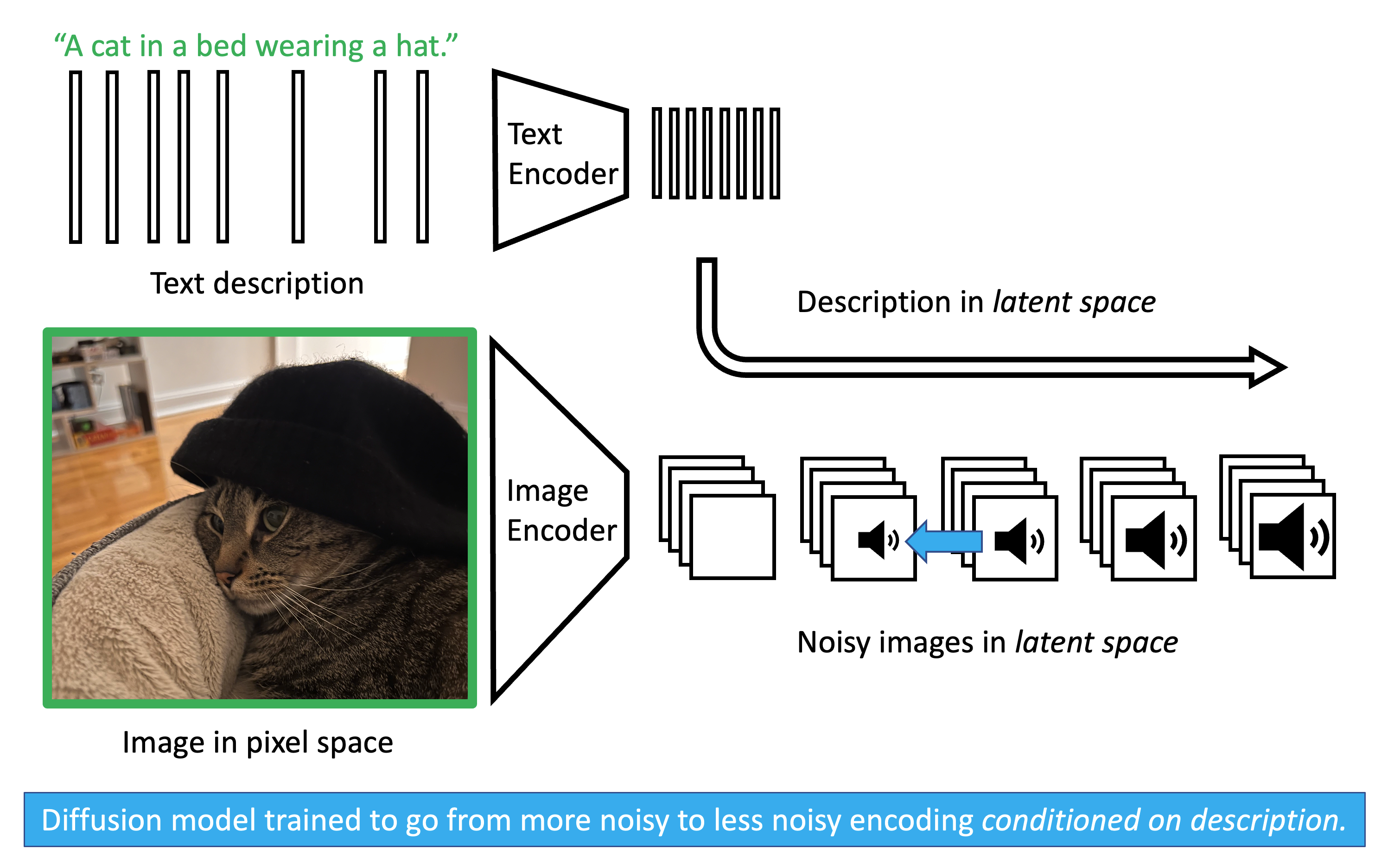
In the training phase, we take images and corresponding text descriptions. For example, we may have an image of a cat in a bed wearing a hat and the text “A cat in a bed wearing a hat.” We encode both the image and text using pretrained variational autoencoders. In the latent space, we add noise to the representation of the image and train a diffusion model to predict the noise that was last applied to each noisy image. Crucially, we also give the diffusion model the latent representation of the text. In this way, the model learns what the latent embedding of an image should look like conditioned on the text description.
I like to think of the text conditioning in the context of watching clouds with a friend. If a friend tells you that a cloud looks like a turtle, your brain starts to see a turtle. In the same way, if we tell a diffusion model that some noise looks like a turtle, the model starts to turn the noise into a turtle.
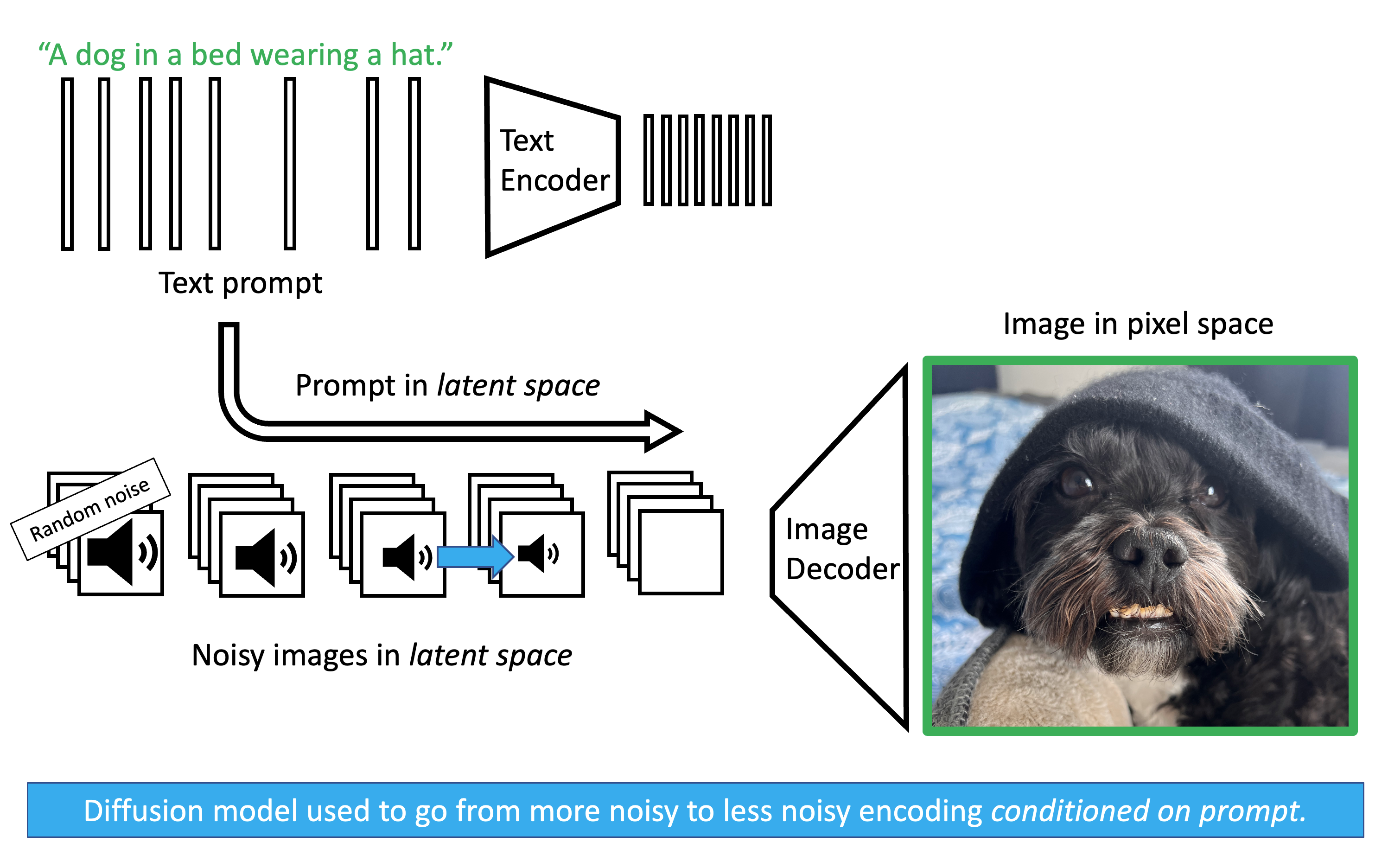
In the testing phase, take a text prompt such as “A dog in a bed wearing a hat.” We encode the text using the pretrained variational text encoder. Then we generate random noise of the same shape as the latent representation of the image in the latent space. Conditioning on the latent representation of the prompt, we use our diffusion model to remove noise from the noisy latent image. When we’re done, we using the decoder of the pretrained image decoder and, with any luck, we produce an image of the text prompt.