Implicit Regularization
Regularization
In this class, we’ll pivot back to the supervised learning setting. We imagine we are given data points \(\mathbf{x} \in \mathbb{R}^d\) and corresponding labels \(y \in \mathbb{R}^d\). The goal is to a build a model \(f_\mathbf{w}: \mathbb{R}^d \rightarrow \mathbb{R}\) where we can choose the weights \(\mathbf{w}\). We will try to find weights so that the model does a good job of fitting the data; that is, we want \(f_\mathbf{w}(\mathbf{x}) \approx \mathbf{y}\).
In order to find these weights, we partition our labelled data into a training set and a validation set. We train and, if all goes well, we find a model that fits the training set. Now the big question is whether the model also fits the validation set. Notice that it is not at all obvious that a model trained on one data set should generalize to another data set. After all, one approach to fitting the training set is simply to memorize it. But, assuming there are lots of models that do fit the training set, there are probably some that generalize well. Our hope is to find these good models.
The first step is to identify what makes some models generalize better than others. Let’s pretend there are two ways to learn: memorize the training set or learn the general concept. If it memorized the training set, the model would output wonky results even for data similar to the training set. If it learned the general concept, the model would output similar results for data similar to the training set. This comparison suggests a desirable property: we want models which produce similar outputs on similar inputs. One way of enforcing this is to reduce the size of each weight. By doing so, we make sure that small changes to the input only lead to small changes in the output. Let’s call such models simple because they’re learning a less ‘sharp’ way of outputting results.
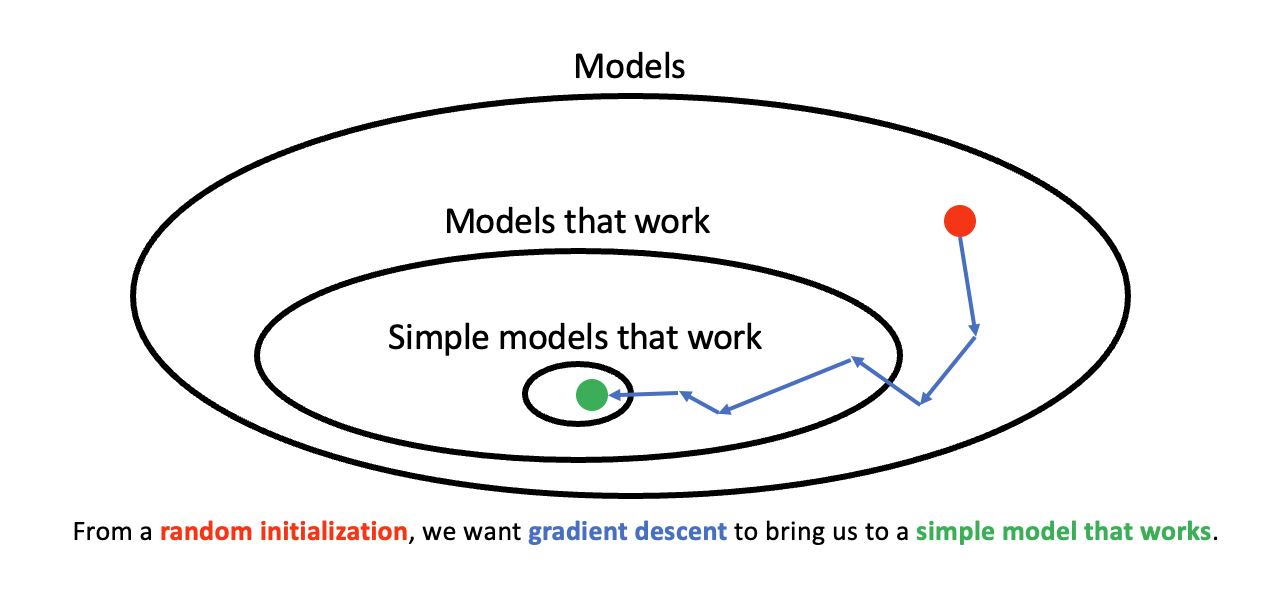
The above figure summarizes our optimistic strategy. We initialize the model with random weights and then update the weights using gradient descent. As we’ve seen again and again, gradient descent will find a model that fits the training set. We hope that the model also fits the validation set. We argued above that such a model should have small norm. One approach of ensuring we find such a model is to use the following loss \[ \mathcal{L}(\mathbf{w}) + \lambda \|\mathbf{w}\|_2^2 \] where \(\mathcal{L}(\mathbf{w})\) is the loss on the training set and \(\lambda\) is a trade off factor. The first term encourages good performance on the training set and the second term encourages simple models. We call this regularization.
Implicit Regularization
If this is how we get models that generalize, why don’t we always use regularization term in our loss? The answer is that the way we train models actually does implicit regularization. In other words, our optimistic strategy is what happens even when we don’t explicitly ask for simple models! Unfortunately, because the math behind neural networks is so complicated, we can’t prove this is what happens in general. But we can prove that implicit regularization happens in several toy examples.
Linear Regression
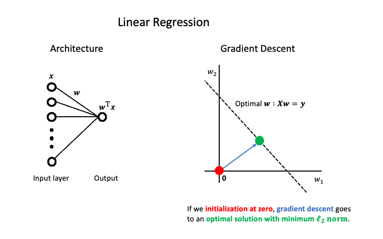
One toy example where we can show that implicit regularization works is linear regression. In this case, the model is given by \(f_\mathbf{w}(\mathbf{x}) = \mathbf{x}^\top \mathbf{w}\) where \(\mathbf{w, x} \in \mathbb{R}^d\). Of course, our goal is to find weights so that the model correctly predicts the labels of points. To this end, our loss function is \[ \mathcal{L}(\mathbf{w}) = \frac{1}{2} \| \mathbf{y} - \mathbf{X w} \|_2^2 \] where \(\mathbf{y} \in \mathbb{R}^n\) is the vector of labels for all \(n\) points in the training set and \(\mathbf{X} \in \mathbb{R}^{n \times d}\) is the data matrix. So that we have lots of optimal solutions, we will assume that \(d > n\). Generally, this so called ‘overparameterized’ setting is standard for neural networks.
We will run gradient descent from a initial weights \(\mathbf{w}_0\). At each step \(t\), we will compute the gradient of the current weights \(\mathbf{w}_t\). Let’s compute the update \[ -\nabla_\mathbf{w} \mathcal{L}(\mathbf{w}_t) = \mathbf{X}^\top (\mathbf{y} - \mathbf{X} \mathbf{w}_t) = \mathbf{X}^\top \pmb{\alpha}_t \] where we defined \(\pmb{\alpha}_t := \mathbf{y} - \mathbf{X} \mathbf{w}_t\). Then, after running for \(T\) iterations, the gradient descent process will output \[ \mathbf{\hat{w}} = \mathbf{w}_0 - \sum_{t=1}^T \nabla_\mathbf{w} \mathcal{L}(\mathbf{w}_t) = \mathbf{w}_0 - \sum_{t=1}^T \mathbf{X}^\top \pmb{\alpha}_t = \mathbf{w}_0 - \mathbf{X}^\top \pmb{\alpha} \] where we defined \(\pmb{\alpha}= \sum_{t=1}^T \pmb{\alpha}_t\). Notice that if we initialize the points at the origin, then we have \(\mathbf{\hat{w}} = \mathbf{X}^\top \pmb{\alpha}\). Equivalently, the output is in the span of the columns of \(\mathbf{X}^\top\). In addition, we can show (see e.g. here) that gradient descent converges to an optimal solution since the linear regression loss is convex. Formally, this means that our output satisfies \(\mathbf{y} = \mathbf{X \hat{w}}\). We now have two equations and two unknowns, let’s solve them for \(\mathbf{\hat{w}}\)! We know \[ \mathbf{y} = \mathbf{X \hat{w}} = \mathbf{X X}^\top \pmb{\alpha} \textrm{ and so } \pmb{\alpha} = \left(\mathbf{X X}^\top\right)^{-1} \mathbf{y}. \] Then, plugging in, we have \[ \mathbf{\hat{w}} = \mathbf{X}^\top \pmb{\alpha} = \mathbf{X} \left(\mathbf{X X}^\top\right)^{-1} \mathbf{y}. \] Now this looks like a strange equation but, as we’ll show momentarily, this is actually the optimal set of weights with minimum \(\ell_2\) norm. Assuming you believe this claim for now, we’ve shown that gradient descent from the origin yields the optimal solution to linear regression with minimum \(\ell_2\) norm. In other words, we have implicit regularization.
Now let’s show that the outputted weights \(\mathbf{\hat{w}}\) have minimum \(\ell_2\) norm. We will consider the problem of finding an optimal solution to the linear regression loss with minimum \(\ell_2\) norm. In particular, we can phrase this as a constrained minimization problem as follows \[ \min_{\mathbf{w}:\mathbf{y}=\mathbf{Xw}} \|\mathbf{w}\|_2 \Longleftrightarrow \min_{\mathbf{w} \in \mathbf{R}^d} \max_{\pmb{\beta} \in \mathbf{R}^n} \|\mathbf{w}\|_2^2 + \pmb{\beta}^\top(\mathbf{y} - \mathbf{Xw}) \] where we reformulated the problem using the method of Lagrange multipliers. The first term encourages regularization while the second term forces \(\mathbf{y}=\mathbf{Wx}\). To see this, notice that if the second term is not the all zeros vector, then \(\pmb{\beta}\) can be arbitrarily large. So, to minimize over weights \(\mathbf{w}\), we better satisfy the constraint that \(\mathbf{y}=\mathbf{Wx}\). The optimal solution to the reformulation is a saddle point. This means that the gradient of the objective with respect to \(\mathbf{w}\) is zero and the gradient of the objective with respect to \(\pmb{\beta}\) is zero. This gives two equations \[ \mathbf{0} = 2 \mathbf{w} - \mathbf{X}^\top \pmb{\beta} \textrm{ and } \mathbf{0} = \mathbf{y} - \mathbf{Xw} \] with two unknowns. As before, let’s solve them! We know \[ \mathbf{w} = \mathbf{X}^\top \pmb{\beta} \frac{1}{2} \textrm{ and } \mathbf{y} = \mathbf{Xw} \textrm{ so } \mathbf{y} = \mathbf{X} \mathbf{X}^\top \pmb{\beta} \frac{1}{2}. \] Then solving for \(\pmb{\beta}\) yields \[ \pmb{\beta} = 2 \left(\mathbf{X}^\top \mathbf{X} \right)^{-1} \mathbf{y} \textrm{ and then } \mathbf{w} = \mathbf{X}^\top \left(\mathbf{X}^\top \mathbf{X} \right)^{-1} \mathbf{y}. \] This is exactly the weights that gradient descent outputs!
Deep Linear Regression
We proved that implicit regularization works in linear regression. But, you may be itching for something deeper. Let’s consider ‘deep linear regression’ where we add more layers but keep them parallel. The architecture appears below.
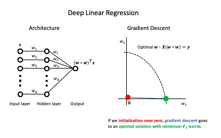
We won’t to prove this but one can show (see e.g. here or the Proof of Appendix D here) that gradient descent yields the optimal weights with minimum \(\ell_1\) norm. Let’s formalize some of the math and then we can wave our hands. As you may expect, the loss is \[ \mathcal{L}(\mathbf{w}) = \| \mathbf{y} - \mathbf{X}(\mathbf{w }\odot \mathbf{w}) \|_2^2 \] where \(\mathbf{w}\odot \mathbf{w}\) denotes entry-wise multiplication. Then the gradient is \[ -\nabla_\mathbf{w} \mathcal{L}(\mathbf{w}) = \mathbf{X}^\top (\mathbf{y} - \mathbf{X} (\mathbf{w} \odot \mathbf{w})) \odot 2 \mathbf{w}. \] The loss looks very similar to before except that we are now multiplying the gradient by its current weights. Intuitively, these updates encourage a rich-get-richer scheme where some weights will grow faster than others. We won’t prove this but, as you can see in this notebook, the gradient pushes the weights toward the minimum \(\ell_1\) norm solution.