Regression MSR
This is a blog post about the paper Regression-adjusted Monte Carlo Estimators for Shapley Values and Probabilistic Values by R. Teal Witter, Yurong Liu, and Christopher Musco.
In the age of complex AI systems, understanding why a model makes a decision is more important than ever. Whether it’s a medical diagnosis, a loan approval, or a hiring recommendation, we need explanations we can trust.
One powerful way to unpack a model’s behavior is through probabilistic values—a family of mathematical tools rooted in game theory. These values quantify how much each feature or data point contributes to a model’s prediction, making them essential in explainable AI.
But there’s a catch: computing these values exactly is infeasible for most real-world models. So, how do we get reliable explanations efficiently?
This post walks through the core ideas behind probabilistic value estimation and introduces our new method—Regression MSR—which offers a powerful, flexible, and statistically grounded approach to model explanations.
🔍 What Are Probabilistic Values?
Imagine trying to assign credit for a model’s prediction to its input features. Probabilistic values do exactly that. They compute the average contribution of each feature by comparing what happens with and without it across various combinations.
Formally, given a value function \(v: 2^{[n]} \to \mathbb{R}\) that maps a subset of features \(S \subseteq [n]\) to the model’s output, we define the probabilistic value for feature \(i \in [n]\) as:
\[ \phi_i(v) = \sum_{S \subseteq [n] \setminus \{i\}} p_{|S|} \cdot \left[ v(S \cup \{i\}) - v(S) \right] \]
The choice of weights \(p_0, \ldots, p_{n-1}\) determine the specific type of probabilistic value:
Shapley values: \(p_{|S|} = \frac{1}{n\binom{n-1}{|S|}}\), which equally weights all subset sizes.
Banzhaf values: \(p_{|S|} = \frac{1}{2^{n-1}}\), which equally weights all subsets.
General probabilistic values: \(p_{|S|}\) can be any non-negative weights that sum to 1, allowing for flexible weighting.
🎲 Method 1: Monte Carlo (MC) Estimation
Monte Carlo is the most straightforward way to estimate probabilistic values: sample subsets randomly, and average the marginal contributions. Here, \(\mathcal{D}(S)\) is the probability density function for the subset \(S\).
\[ \tilde{\phi}_i^{\text{MC}} = \frac{1}{|\mathcal{S}_i|} \sum_{S \in \mathcal{S}_i} \left[ v(S \cup \{i\}) - v(S) \right] \cdot \frac{p_{|S|}}{\mathcal{D}(S)} \]
✅ Unbiased
❌ No sample reuse, each feature’s value requires separate samples.
❌ High variance, depends on \([v(S \cup \{i\}) - v(S)]^2\).
✅ Generalizable, works for any probabilistic value.
♻️ Method 2: Maximum Sample Reuse (MSR)
MSR improves sample efficiency by reusing the same subsets \(\mathcal{S}\) across all features.
\[ \tilde{\phi}_i^{\text{MSR}} = \frac{1}{|\mathcal{S}|} \sum_{S \in \mathcal{S}} v(S) \cdot \frac{p_{|S|-1} \cdot \mathbb{1}[i \in S] - p_{|S|} \cdot \mathbb{1}[i \notin S]}{\mathcal{D}(S)} \]
✅ Unbiased
✅ Sample reuse
❌ Very high variance, depends on \(v(S)^2\).
✅ Generalizable
MSR offers a big efficiency boost, but it generally doesn’t reduce variance.
📈 Method 3: Regression-Based Estimators
Shapley values can also be framed as the solution to a linear regression problem.
\[ \begin{bmatrix} \phi_1 \\ \vdots \\ \phi_n \end{bmatrix} = \arg \min_{\mathbf{x} \in \mathbb{R}^n: \langle \mathbf{x}, \mathbf{1} \rangle = v([n])} \sum_{S \subseteq [n]} \frac{\left( v(S) - \sum_{i \in S} x_i \right)^2}{\binom{n}{|S|}|S|(n-|S|)} \]
This regression formulation leads to:
- Kernel SHAP: the most popular linear regression-based method.
- Leverage SHAP: samples more intelligently using leverage scores, prior state-of-the-art for Shapley value estimation.
❌ Biased
✅ Sample reuse
✅ Low variance
❌ Not generalizable, requires special regression formulations for each probabilistic value.
Linear regression-based methods are powerful, but they are limited based on how well the linear model captures the value function \(v\). They also require custom formulations for each type of probabilistic value, which can be cumbersome.
🎯 Our Contribution: Regression MSR
We introduce Regression MSR—a method that blends the strengths of regression and MSR, while avoiding their weaknesses.
💡 Key Idea
We approximate the value function \(v\) with a simpler model \(f\) (e.g., a linear model or a decision tree, where we can efficiently compute the probabilistic values). Then, because probabilistic values are linear:
\[ \phi_i(v) = \phi_i(f) + \phi_i(v - f) \]
We use MSR to estimate \(\phi_i(v - f)\), and compute \(\phi_i(f)\) exactly.
\[ \tilde{\phi}_i^{\text{RegMSR}} = \phi_i(f) + \frac{1}{|\mathcal{S}|} \sum_{S \in \mathcal{S}} [v(S) - f(S)] \cdot \frac{p_{|S|-1} \mathbb{1}[i \in S] - p_{|S|} \mathbb{1}[i \notin S]}{\mathcal{D}(S)} \]
✅ Unbiased
✅ Sample reuse
✅ Low variance, depends on \([v(S) - f(S)]^2\).
✅ General
We call this estimator Regression MSR. We explore two strategies for learning the function \(f\):
📏 Linear MSR Use a linear model. Fast to compute, may not capture complex relationships.
🌲 Tree MSR Fit a decision tree or ensemble (like XGBoost) to approximate \(v\). We develop an efficient algorithm for computing probabilistic values of trees—extending prior work on Shapley/Banzhaf values.
🔧 Practical Considerations
A straightforward way to implement Regression MSR is to train the function \(f\) and compute the final estimates using the same set of samples. While this often yields accurate results in practice, it introduces a small bias because the same data is used both to fit the model and to evaluate it.
To make the estimator unbiased, we use a \(k\)-fold sample-splitting strategy:
- Divide the samples into \(k\) equal parts (folds).
- For each fold, train \(f\) on the other \(k-1\) folds and compute the estimate using the held-out fold.
- Repeat this process \(k\) times so that all samples are used, but never for both training and estimation simultaneously.
This ensures that the training and estimation stages remain independent, which removes bias and enables a clean calculation of the estimator’s variance (as described in the paper). In our experiments, we use \(k=10\), so that each fold has enough samples to provide a reliable estimate while still allowing for efficient computation. For settings where a small bias (like that of Kernel SHAP or Leverage SHAP) is acceptable, we recommend using the same samples for both training and estimation.
📊 Experimental Highlights (Estimating Shapley Values)
Performance
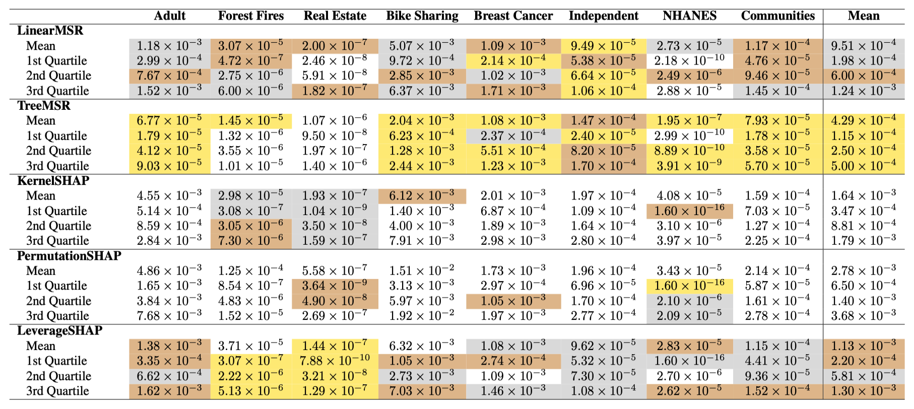
Tree MSR Shapley value estimates with average error that is \(6.5\times\) lower than Permutation SHAP (the most popular Monte Carlo method), \(3.8\times\) lower than Kernel SHAP (the most popular linear regression method), and \(2.6\times\) lower than Leverage SHAP (the prior state-of-the-art Shapley value estimator).
Sample Complexity
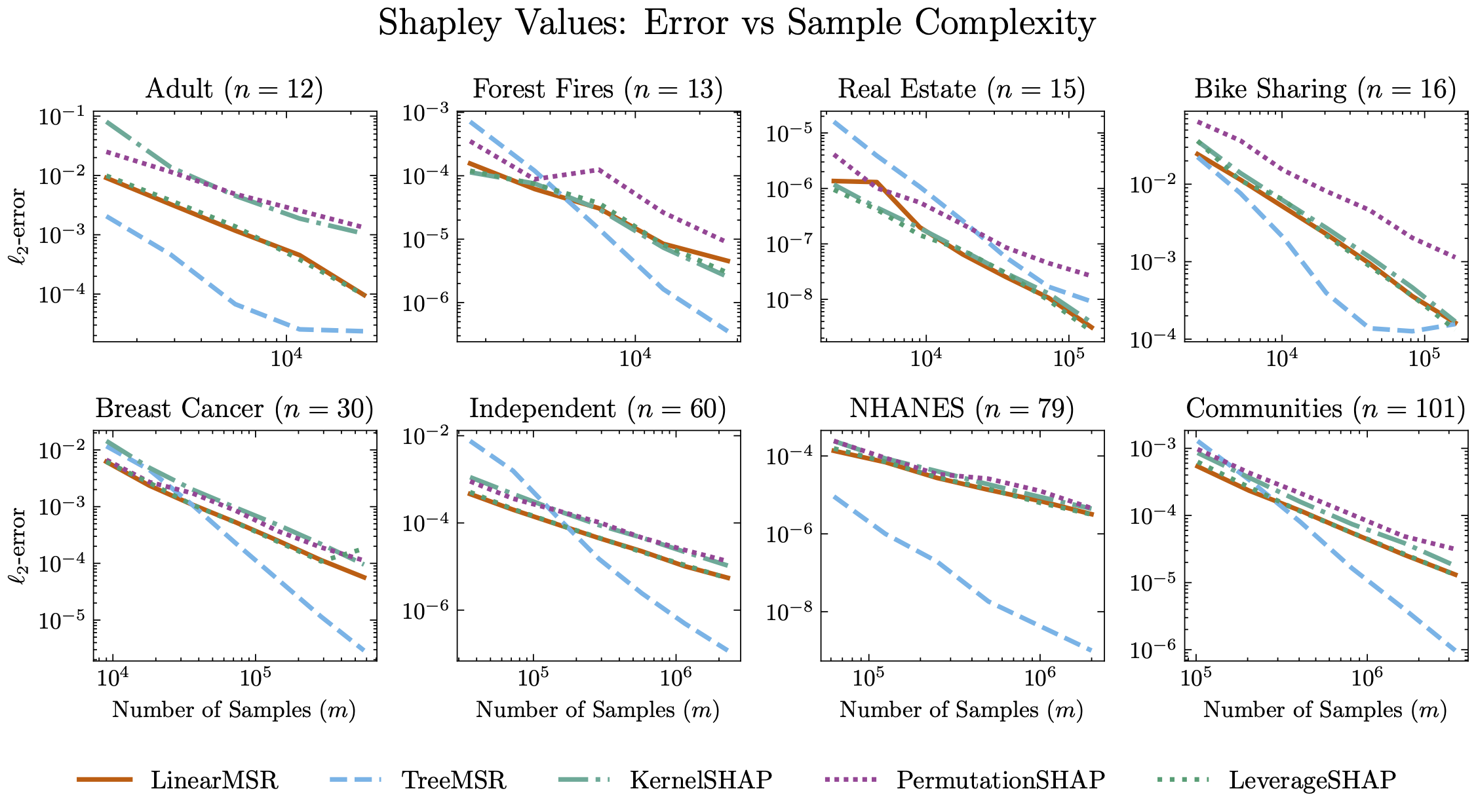
As the number of samples increases, Tree MSR continues to improve, generally outpacing even the best regression-based estimators like Leverage SHAP.
For more details, please check out the full paper on arXiv. And, feel free to reach out!
This post was generated with the help of ChatGPT.