Trace Estimation with Hutch++
9 min read
Our topic today combines two of my favorite technical ideas:
Outer products. In my teaching, I like to write a matrix as a sum of outer products of its eigenvectors. This lets us understand the matrix one direction at a time: each term picks out an eigenvector’s direction and scales it by the corresponding eigenvalue. Ideas like the power method and low-rank approximation become much easier to see.
Control variates. In my research, I often want to estimate a quantity using as few queries as possible. A useful starting point is an approximation whose contribution I can compute exactly. Then I only have to estimate the correction. I’ve used this idea to estimate Shapley values with algorithms like Regression MSR.
These two ideas come together in trace estimation: estimating the sum of diagonal entries in a square matrix. The algorithm we’ll study, Hutch++, is the work of Raphael Meyer, Cameron Musco, Chris Musco, and David Woodruff. Chris was my PhD advisor, Raphael is a former student of his, and Cameron is Chris’s brother. Chris and Raphael shaped my PhD, so this algorithm is one of my favorites.
Linear Algebra Fun
For simplicity, we’ll assume our matrix \(\mathbf{A} \in \mathbb{R}^{d \times d}\) is nonzero, symmetric, and positive semidefinite (PSD). Let \(\lambda_1 \geq \lambda_2 \geq \cdots \geq \lambda_d \geq 0\) be its eigenvalues, with corresponding eigenvectors \(\mathbf{v}_1, \ldots, \mathbf{v}_d \in \mathbb{R}^d\). We can choose these eigenvectors to be orthonormal: \(\mathbf{v}_i^\top \mathbf{v}_j\) is \(1\) if \(i=j\) and \(0\) otherwise. The familiar eigenvector identity, \(\mathbf{A}\mathbf{v}_i = \lambda_i\mathbf{v}_i\), says that along each eigenvector, the matrix acts by simple scaling. The outer-product representation writes these actions separately and adds them together.
Outer-product view. A symmetric matrix can be written as
\[ \mathbf{A} = \sum_{i=1}^d \lambda_i\mathbf{v}_i\mathbf{v}_i^\top. \]
Proof
Apply the matrix on the right to any eigenvector \(\mathbf{v}_j\):
\[ \left(\sum_{i=1}^d \lambda_i\mathbf{v}_i\mathbf{v}_i^\top\right)\mathbf{v}_j = \lambda_j\mathbf{v}_j = \mathbf{A}\mathbf{v}_j. \]
The two matrices agree on every vector in a basis, so they are equal.
To connect this view to the trace, let’s start with its definition as the sum of diagonal entries:
\[ \operatorname{tr}(\mathbf{A}) = \sum_{i=1}^d [\mathbf{A}]_{i,i}. \]
Since the trace is a sum of entries, it respects addition and scalar multiplication. It also has a cyclic property: we can swap the order of two factors inside the trace, even when the factors are rectangular.
Cyclic trace. For \(\mathbf{X} \in \mathbb{R}^{n \times d}\) and \(\mathbf{Y} \in \mathbb{R}^{d \times n}\),
\[ \operatorname{tr}(\mathbf{X}\mathbf{Y}) = \operatorname{tr}(\mathbf{Y}\mathbf{X}). \]
Proof
Expand the diagonal entries and switch the order of summation:
\[ \begin{aligned} \operatorname{tr}(\mathbf{X}\mathbf{Y}) &= \sum_{i=1}^n \sum_{j=1}^d [\mathbf{X}]_{i,j}[\mathbf{Y}]_{j,i} \\ &= \sum_{j=1}^d \sum_{i=1}^n [\mathbf{Y}]_{j,i}[\mathbf{X}]_{i,j} \\ &= \operatorname{tr}(\mathbf{Y}\mathbf{X}). \end{aligned} \]
Now apply this property to each outer product. The trace of each term is just its eigenvalue, so adding the terms gives another expression for the trace.
Trace as an eigenvalue sum.
\[ \operatorname{tr}(\mathbf{A}) = \sum_{i=1}^d \lambda_i. \]
Proof
By linearity, cyclicity, and the fact that each eigenvector has length one,
\[ \begin{aligned} \operatorname{tr}(\mathbf{A}) &= \sum_{i=1}^d \lambda_i\operatorname{tr}(\mathbf{v}_i\mathbf{v}_i^\top) \\ &= \sum_{i=1}^d \lambda_i\operatorname{tr}(\mathbf{v}_i^\top\mathbf{v}_i) \\ &= \sum_{i=1}^d \lambda_i. \end{aligned} \]
For a covariance matrix, these two expressions have a familiar meaning: the diagonal entries are the variances of the individual coordinates, and the eigenvalues are the variances along the principal components. Either way, their sum gives the total variance. Traces also appear in Gaussian likelihoods through the log-determinant: for a positive definite matrix \(\mathbf{B}\), \(\log\det(\mathbf{B}) = \operatorname{tr}(\log\mathbf{B})\). (Here \(\log\mathbf{B}\) need not be PSD, so our relative-error guarantee won’t always apply.)
We’ll also need the Frobenius norm to measure the error of our estimates. Its square, \(\|\mathbf{A}\|_{\mathrm F}^2\), is the sum of squared entries, which we can also write as a trace.
Frobenius norm as a trace.
\[ \|\mathbf{A}\|_{\mathrm F}^2 = \sum_{i=1}^d\sum_{j=1}^d [\mathbf{A}]_{i,j}^2 = \operatorname{tr}(\mathbf{A}^\top\mathbf{A}). \]
Proof
Write out the diagonal entries of the product:
\[ \begin{aligned} \operatorname{tr}(\mathbf{A}^\top\mathbf{A}) &= \sum_{j=1}^d\sum_{i=1}^d [\mathbf{A}^\top]_{j,i}[\mathbf{A}]_{i,j} \\ &= \sum_{j=1}^d\sum_{i=1}^d [\mathbf{A}]_{i,j}^2 \\ &= \|\mathbf{A}\|_{\mathrm F}^2. \end{aligned} \]
One last connection, I promise: the squared Frobenius norm is also the sum of squared eigenvalues.
Frobenius norm as an eigenvalue sum. For symmetric \(\mathbf{A}\),
\[ \|\mathbf{A}\|_{\mathrm F}^2 = \sum_{i=1}^d \lambda_i^2. \]
Proof
By symmetry and the orthonormality of the eigenvectors,
\[ \begin{aligned} \mathbf{A}^\top\mathbf{A} &= \left(\sum_{i=1}^d \lambda_i\mathbf{v}_i\mathbf{v}_i^\top\right) \left(\sum_{j=1}^d \lambda_j\mathbf{v}_j\mathbf{v}_j^\top\right) \\ &= \sum_{i=1}^d \lambda_i^2\mathbf{v}_i\mathbf{v}_i^\top. \end{aligned} \]
Taking the trace gives \(\|\mathbf{A}\|_{\mathrm F}^2 = \sum_{i=1}^d \lambda_i^2\). A similar expansion of \(\mathbf{A}^k\) explains the power method: raising the eigenvalues to the \(k\)th power makes the largest ones more prominent relative to the others.
We can now use these identities to analyze a trace estimate.
Hutchinson’s Estimator
Suppose we can access \(\mathbf{A}\) only through matrix-vector products: we choose a vector \(\mathbf{x} \in \mathbb{R}^d\) and receive \(\mathbf{A}\mathbf{x}\). For example, \(\mathbf{A}\) might be the inverse of a matrix we store. We can apply that inverse to a vector by solving a linear system, without forming the inverse itself.
Our budget is \(m\) queries. With \(d\) queries, we could apply \(\mathbf{A}\) to each standard basis vector and read off the diagonal entries exactly. So the game is getting a good approximation with \(m \ll d\).
Draw a random vector \(\mathbf{z} \in \{-1,1\}^d\) whose entries \(z_1,\ldots,z_d\) are independent fair signs, also called Rademacher random variables. One matrix-vector product, followed by a dot product, gives
\[ \begin{aligned} \mathbf{z}^\top\mathbf{A}\mathbf{z} &= \sum_{i=1}^d\sum_{j=1}^d [\mathbf{A}]_{i,j}z_i z_j \\ &= \sum_{i=1}^d [\mathbf{A}]_{i,i}z_i^2 + 2\sum_{i=1}^{d-1}\sum_{j=i+1}^d [\mathbf{A}]_{i,j}z_i z_j \\ &= \operatorname{tr}(\mathbf{A}) + 2\sum_{i=1}^{d-1}\sum_{j=i+1}^d [\mathbf{A}]_{i,j}z_i z_j. \end{aligned} \]
Symmetry lets us pair up the off-diagonal terms, while \(z_i^2=1\) preserves every diagonal entry. The remaining terms have mean zero: independence gives \(\mathbb{E}[z_i z_j]=0\) for \(i\ne j\). Taking the expectation leaves exactly the trace.
Repeating \(m\) times with independent vectors \(\mathbf{z}_1,\ldots,\mathbf{z}_m\) and averaging gives Hutchinson’s estimator:
\[ \widehat{\operatorname{tr}}^{\,\mathrm h}_m(\mathbf{A}) = \frac{1}{m}\sum_{j=1}^m \mathbf{z}_j^\top\mathbf{A}\mathbf{z}_j. \]
The same expansion gives the variance. The diagonal contributes no randomness; the off-diagonal entries determine how much each probe fluctuates.
Hutchinson’s mean and variance. For symmetric \(\mathbf{A}\),
\[ \mathbb{E}\!\left[\widehat{\operatorname{tr}}^{\,\mathrm h}_m(\mathbf{A})\right] = \operatorname{tr}(\mathbf{A}), \]
\[ \operatorname{Var}\!\left(\widehat{\operatorname{tr}}^{\,\mathrm h}_m(\mathbf{A})\right) = \frac{4}{m}\sum_{i=1}^{d-1}\sum_{j=i+1}^d [\mathbf{A}]_{i,j}^2 \le \frac{2}{m}\|\mathbf{A}\|_{\mathrm F}^2. \]
Proof
We’ve already shown unbiasedness. For the variance, each \(z_i z_j\) with \(i<j\) has mean zero and square one. Different pairs are uncorrelated, even if they share an index: their product contains at least one sign that appears only once, so its expectation is zero. Thus,
\[ \begin{aligned} \operatorname{Var}(\mathbf{z}^\top\mathbf{A}\mathbf{z}) &= 4\sum_{i=1}^{d-1}\sum_{j=i+1}^d [\mathbf{A}]_{i,j}^2 \\ &\le 2\sum_{i=1}^d\sum_{j=1}^d [\mathbf{A}]_{i,j}^2 \\ &= 2\|\mathbf{A}\|_{\mathrm F}^2. \end{aligned} \]
Averaging \(m\) independent estimates divides the variance by \(m\).
We can now apply Chebyshev’s inequality:
\[ \Pr\!\left( \left|\widehat{\operatorname{tr}}^{\,\mathrm h}_m(\mathbf{A})-\operatorname{tr}(\mathbf{A})\right| \geq \varepsilon\operatorname{tr}(\mathbf{A}) \right) \leq \frac{2\|\mathbf{A}\|_{\mathrm F}^2} {m\varepsilon^2\operatorname{tr}(\mathbf{A})^2}. \]
To see when this bound is small, compare the Frobenius norm with the trace. Our eigenvalue identities give
\[ \frac{\|\mathbf{A}\|_{\mathrm F}}{\operatorname{tr}(\mathbf{A})} = \frac{\sqrt{\sum_{i=1}^d\lambda_i^2}}{\sum_{i=1}^d\lambda_i} \leq 1. \]
The numerator is the \(\ell_2\) norm of the eigenvalues, and the denominator is their \(\ell_1\) norm: their sum, since they’re nonnegative. The ratio is at most one, so taking \(m\) to be a sufficiently large constant times \(1/\varepsilon^2\) makes the failure probability at most \(1/10\).
We get a better bound when the spectrum is flat, meaning the eigenvalues are all close: the ratio is then about \(1/\sqrt{d}\). If one eigenvalue dominates the sum, the ratio approaches one and we lose that advantage. The exact variance still depends on the off-diagonal entries; for a diagonal matrix, even one probe gives the trace exactly.
Hutch++ uses a low-rank approximation to account for the largest eigenvalues before sampling the rest.
Control Variate
Suppose we could learn an approximation \(\mathbf{B}\) whose trace is easy to compute. We could account for that part exactly and use Hutchinson’s estimator only on the difference, \(\mathbf{A}-\mathbf{B}\). By linearity,
\[ \widehat{\operatorname{tr}}(\mathbf{A}) = \operatorname{tr}(\mathbf{B}) + \widehat{\operatorname{tr}}^{\,\mathrm h}_m(\mathbf{A}-\mathbf{B}). \]
The first term is exact, so the residual determines the error. For a fixed symmetric \(\mathbf{B}\), Hutchinson’s variance bound gives
\[ \operatorname{Var}\!\left(\widehat{\operatorname{tr}}(\mathbf{A})\right) \leq \frac{2}{m}\|\mathbf{A}-\mathbf{B}\|_{\mathrm F}^2. \]
We’d like an approximation that’s simple to represent and leaves a small residual. Among matrices of rank at most \(k\), the Eckart–Young theorem tells us to keep the terms corresponding to the \(k\) largest eigenvalues:
\[ \mathbf{A}_k = \sum_{i=1}^k \lambda_i\mathbf{v}_i\mathbf{v}_i^\top. \]
If we knew these eigenvalues and eigenvectors, the trace of \(\mathbf{A}_k\) would simply be \(\sum_{i=1}^k\lambda_i\). The residual contains the remaining terms. Our Frobenius norm identity expresses its size as a sum of squared eigenvalues, which we can bound using the trace.
Low-rank residual bound. For PSD \(\mathbf{A}\) and \(1\leq k<d\),
\[ \|\mathbf{A}-\mathbf{A}_k\|_{\mathrm F}^2 = \sum_{i=k+1}^d\lambda_i^2 \leq \frac{\operatorname{tr}(\mathbf{A})^2}{k}. \]
Proof
Each of the top \(k\) eigenvalues is at least \(\lambda_{k+1}\), so
\[ \lambda_{k+1} \leq \frac{1}{k}\sum_{i=1}^k\lambda_i \leq \frac{\operatorname{tr}(\mathbf{A})}{k}. \]
Every remaining eigenvalue is at most \(\lambda_{k+1}\). Therefore,
\[ \begin{aligned} \|\mathbf{A}-\mathbf{A}_k\|_{\mathrm F}^2 &= \sum_{i=k+1}^d\lambda_i^2 \\ &\leq \lambda_{k+1}\sum_{i=k+1}^d\lambda_i \\ &\leq \frac{\operatorname{tr}(\mathbf{A})}{k}\sum_{i=k+1}^d\lambda_i \\ &\leq \frac{\operatorname{tr}(\mathbf{A})^2}{k}. \end{aligned} \]
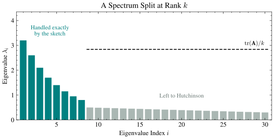
Plugging this into Chebyshev’s inequality gives, for the ideal choice \(\mathbf{B}=\mathbf{A}_k\),
\[ \Pr\!\left( \left|\widehat{\operatorname{tr}}(\mathbf{A})-\operatorname{tr}(\mathbf{A})\right| \geq \varepsilon\operatorname{tr}(\mathbf{A}) \right) \leq \frac{2}{mk\varepsilon^2}. \]
If \(k\) grows proportionally with \(m\), the denominator grows as \(m^2\varepsilon^2\). That would let us reach the same constant failure probability with \(m\) proportional to \(1/\varepsilon\). We still have to account for the queries used to find the approximation. Finding the top eigenvectors exactly is generally too expensive, but we only need to approximate their span.
Hutch++
Hutch++ spends two thirds of its \(m\) queries learning a structured approximation \(\mathbf{B}\) and computing its trace exactly. It finds the approximation by multiplying random vectors by \(\mathbf{A}\), which emphasizes the directions associated with large eigenvalues. The remaining third of the queries uses Hutchinson’s estimator to estimate the trace of \(\mathbf{A}-\mathbf{B}\). We use fresh random vectors for this step and add the estimate to \(\operatorname{tr}(\mathbf{B})\).
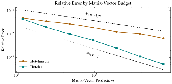
We don’t need to find the top eigenvectors exactly for this to work. The Hutch++ analysis shows that this approximation is accurate enough to preserve the improvement we just derived: \(O(1/\varepsilon)\) queries give relative error at most \(\varepsilon\) with constant success probability, compared with \(O(1/\varepsilon^2)\) for Hutchinson’s estimator. The plot below compares their errors at the same query budget.