The Gumbel Sampling Trick
4 min read
Suppose a model assigns three options probabilities \(0.6\), \(0.3\), and \(0.1\). Taking the largest probability always returns the first option. Sampling should return it only sixty percent of the time. Can we turn a maximum into an exact random sample by adding noise?
Yes, with a particular kind of noise called Gumbel noise. The useful part is not just that lower-scoring options sometimes win. We can prove exactly how often each option wins.
Add Noise, Then Choose
Write \(s_1,\ldots,s_n\) for the model’s scores, or logits. At temperature \(b>0\), the desired probabilities are
\[\begin{align*} p_i=\frac{e^{s_i/b}}{\sum_{j=1}^n e^{s_j/b}}. \end{align*}\]
Small temperatures concentrate probability on the best scores. Large temperatures make the probabilities more even. To get the opening example at \(b=1\), take \(s=(\log0.6,\log0.3,\log0.1)\).
Draw independent standard Gumbel variables \(G_1,\ldots,G_n\), and return
\[\begin{align*} I=\arg\max_{1\le i\le n}\{s_i+bG_i\}. \end{align*}\]
Each option gets its own noise draw. Adding one shared draw to every score would leave the winner unchanged.
Chance of winning
We can generate a standard Gumbel from a uniform draw \(U\in(0,1)\) by setting \(G=-\log(-\log U)\). Its cumulative distribution function is
\[\begin{align*} F(t)=\Pr(G\le t)=\exp(-e^{-t}). \end{align*}\]
This unusual-looking function is precisely what makes the winning probabilities simple.
Why the Winner Has the Right Distribution
First divide all perturbed scores by \(b\), which leaves their ordering unchanged. For candidate \(i\) to win with noise \(G_i=t\), every rival must satisfy \(G_j\le t+(s_i-s_j)/b\). Independence lets us multiply those probabilities.
Gumbel-max trick: With independent standard Gumbel draws,
\[\begin{align*} \Pr(I=i)=\frac{e^{s_i/b}}{\sum_{j=1}^n e^{s_j/b}}. \end{align*}\]
Proof
A shift in the Gumbel cumulative distribution becomes a power:
\[\begin{align*} F(t+c)=\exp(-e^{-t}e^{-c})=F(t)^{e^{-c}}. \end{align*}\]
Fixing \(G_i=t\), multiply the chances of beating each rival:
\[\begin{align*} \Pr(I=i\mid G_i=t) =\prod_{j\ne i}F\!\left(t+\frac{s_i-s_j}{b}\right) =F(t)^{\sum_{j\ne i}e^{(s_j-s_i)/b}}. \end{align*}\]
Now average over \(G_i\). The change of variables \(u=F(t)\) turns its density \(f(t)\,dt\) into \(du\):
\[\begin{align*} \Pr(I=i) &=\int_0^1u^{\sum_{j\ne i}e^{(s_j-s_i)/b}}\,du\\ &=\frac{1}{1+\sum_{j\ne i}e^{(s_j-s_i)/b}} =\frac{e^{s_i/b}}{\sum_{j=1}^n e^{s_j/b}}. \end{align*}\]
Ties have probability zero because the noise is continuous.
The noise turns maximization into sampling from softmax. In particular, choosing \(s_i=\log p_i\) and \(b=1\) samples from any categorical distribution \(p\). Tokens with \(p_i=0\) can simply be omitted. The connection between Gumbel noise and choice probabilities is classical Yellott, 1977.
There is also a useful second view. If \(E_i\sim\mathrm{Exp}(1)\), then \(G_i=-\log E_i\) is standard Gumbel, so
\[\begin{align*} \arg\max_i\{\log p_i+G_i\} =\arg\min_i\frac{E_i}{p_i}. \end{align*}\]
The largest perturbed log-probability and the earliest exponential arrival select the very same token.
What If We Use a Different Noise?
The choice of noise determines the distribution of the winner. Consider just two scores, \(g\) and \(0\), where \(g\ge0\) is their gap. For Gumbel noise with scale \(b\), the lower score wins with probability \(1/(1+e^{g/b})\).
Independent exponential or Laplace noise of scale \(b\) gives different answers:
| Noise added to each score | Chance the lower score wins |
|---|---|
| Gumbel | \(\displaystyle\frac{1}{1+e^{g/b}}\) |
| Exponential | \(\displaystyle\frac12e^{-g/b}\) |
| Laplace | \(\displaystyle\frac14(g/b+2)e^{-g/b}\) |
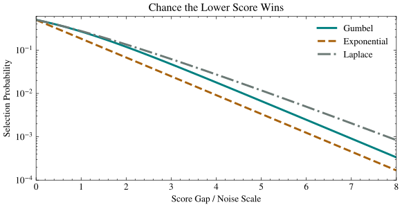
Only the ratio \(g/b\) matters. At a tie, each option wins half the time under every rule. As the gap grows, the noise distributions disagree about how often to choose the lower score. These are equal scale parameters, not equal variances.
Deriving the other two probabilities
If the lower option’s noise is \(t\), the leader’s must be below \(t-g\). For a common noise density \(f\) and cumulative distribution \(F\), this gives
\[\begin{align*} \Pr(\text{lower wins})=\int_{-\infty}^{\infty}f(t)F(t-g)\,dt. \end{align*}\]
Exponential noise is nonnegative, so the lower option must first clear \(g\). For \(t\ge0\), its density is \(e^{-t/b}/b\) and its cumulative distribution is \(1-e^{-t/b}\). Thus
\[\begin{align*} \Pr(\text{lower wins}) =\int_g^\infty\frac{e^{-t/b}}b\left(1-e^{-(t-g)/b}\right)dt =\frac12e^{-g/b}. \end{align*}\]
Laplace noise has density \(e^{-|t|/b}/(2b)\). Its cumulative distribution is \(e^{t/b}/2\) for \(t<0\) and \(1-e^{-t/b}/2\) for \(t\ge0\). Splitting the same integral at \(0\) and \(g\) gives
\[\begin{align*} \Pr(\text{lower wins}) =\left(\frac18+\frac{g}{4b}+\frac38\right)e^{-g/b}. \end{align*}\]
The middle term comes from \(0<t<g\): a positive draw for the lower option and a negative draw for the leader can share the work of closing the gap.
From Sampling to Private Selection
Suppose the scores depend on people’s data, and changing one person’s record changes each score by at most \(\Delta>0\). A deterministic maximum can change abruptly. Randomized selection lets us control how much the output probabilities change.
For Gumbel noise, choose \(b=2\Delta/\varepsilon\). On neighboring datasets, the numerator \(e^{s_i/b}\) changes by at most a factor \(e^{\Delta/b}\), and so does the denominator. The probability of returning any particular index therefore changes by at most
\[\begin{align*} e^{2\Delta/b}=e^\varepsilon. \end{align*}\]
This is \(\varepsilon\)-differential privacy for the released index. The resulting softmax rule is called the exponential mechanism, after its exponential weights. It uses Gumbel noise, despite the name.
Exponential and Laplace noise also give privacy at this same sufficient scale Ding et al., 2021. Thus the comparison above also compares three rules with a common privacy guarantee. For two options, exponential noise selects the lower score less often than Gumbel noise whenever the gap is positive. The more general result is that it has no larger expected score loss, for any number of candidates McKenna and Sheldon, 2020.
Why exponential noise is also called permute-and-flip
Subtract the largest score from every score, so the best is zero. A candidate \(i\) with exponential noise \(Z_i\) reaches zero with probability \(e^{s_i/b}\). These events are independent, and at least one best candidate always reaches zero.
Conditional on reaching zero, memorylessness gives
\[\begin{align*} \Pr(s_i+Z_i>x\mid Z_i\ge-s_i)=e^{-x/b},\qquad x\ge0. \end{align*}\]
The excesses above zero are independent and identically distributed. Conditional on which candidates reach zero, each is therefore equally likely to have the largest excess.
We can get the same winner distribution by marking each candidate independently with probability \(e^{s_i/b}\), shuffling the candidates uniformly, and returning the first marked one. This is permute-and-flip, equivalent to exponential noisy argmax Ding et al., 2021.
Gumbel noise answers the original question exactly: maximization can sample from prescribed probabilities. Other noises give different selection rules, which can be useful when the goal is to choose a good option privately.